Estimation of expected annual damage, EAD

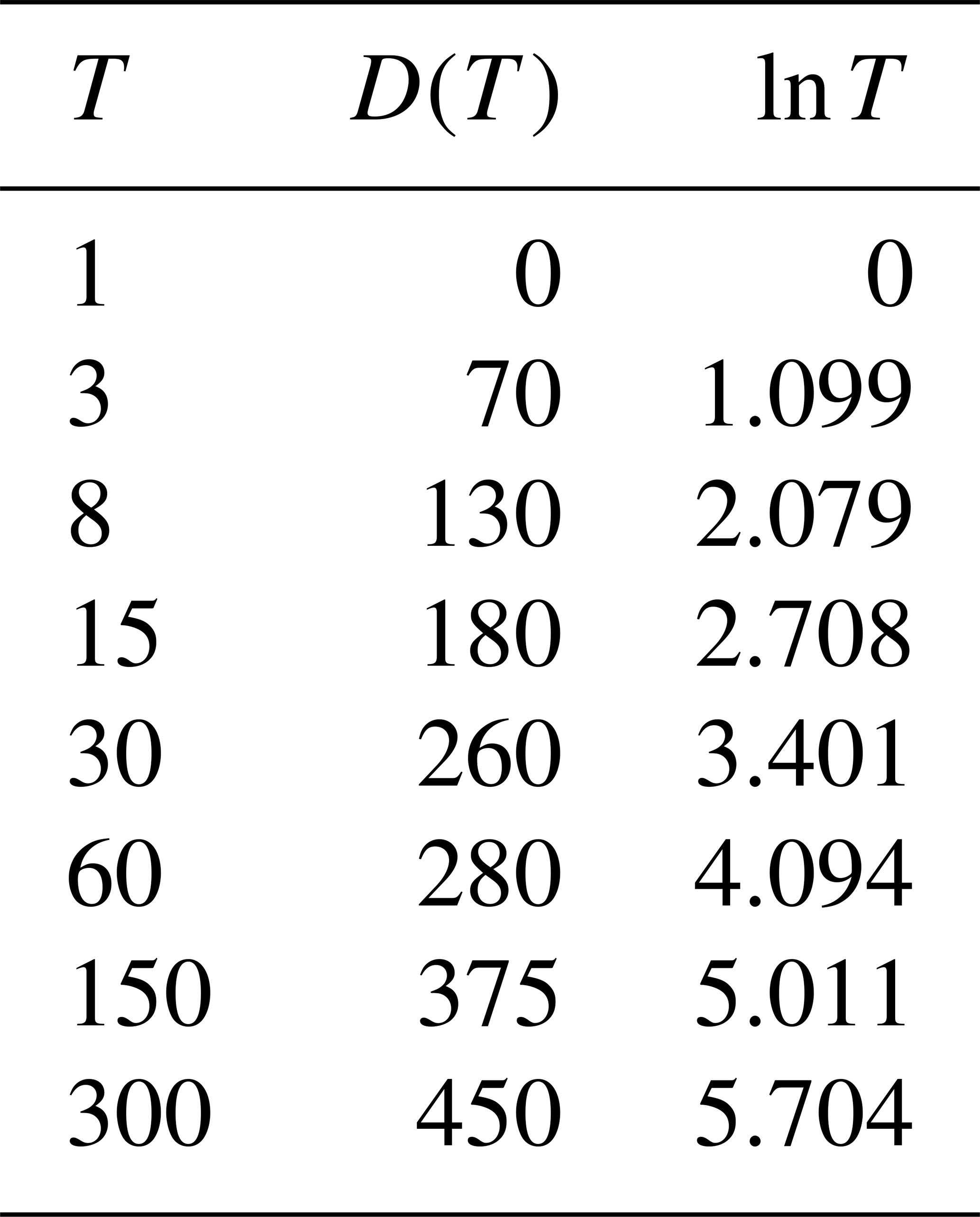
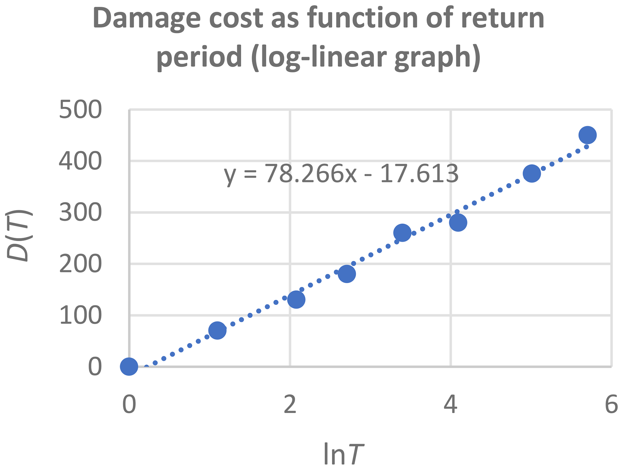
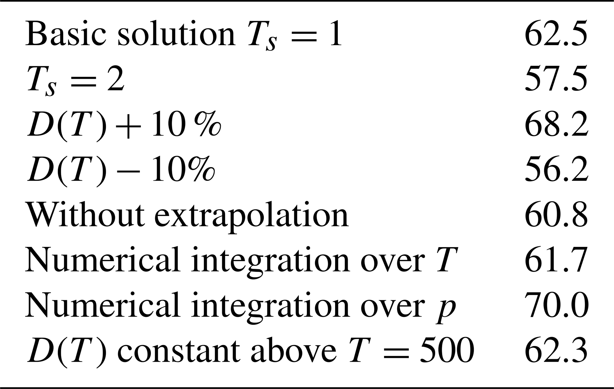
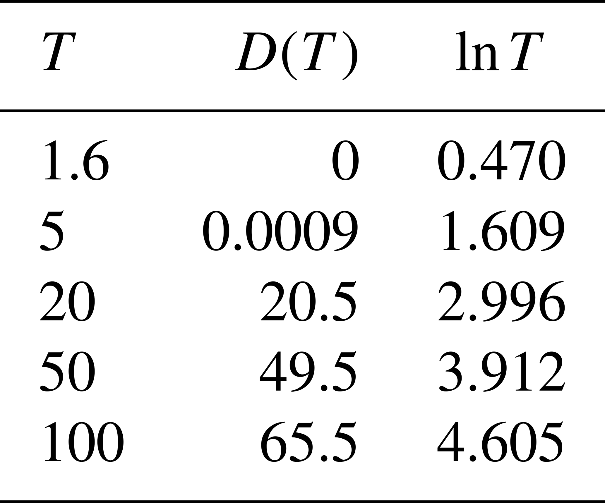
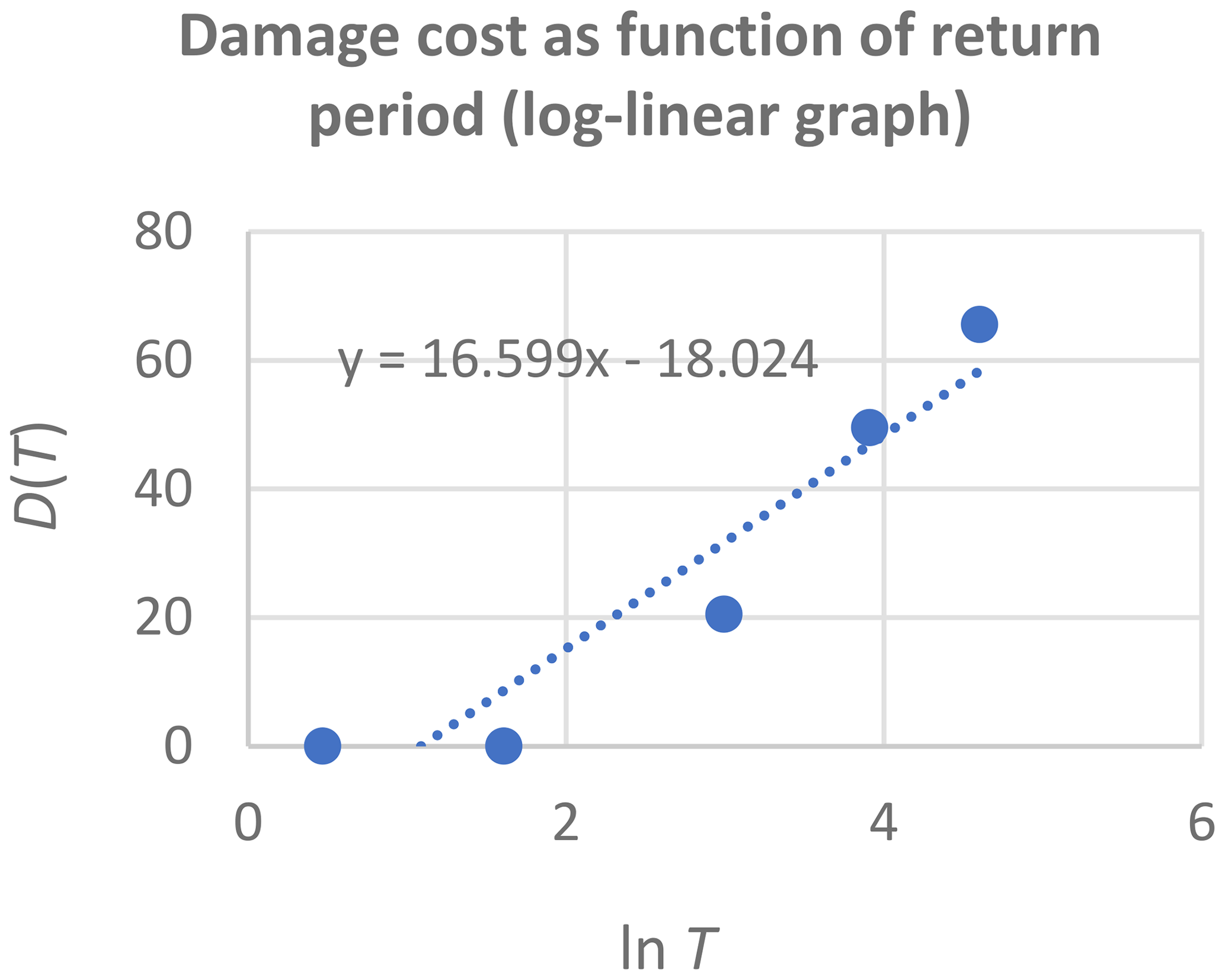
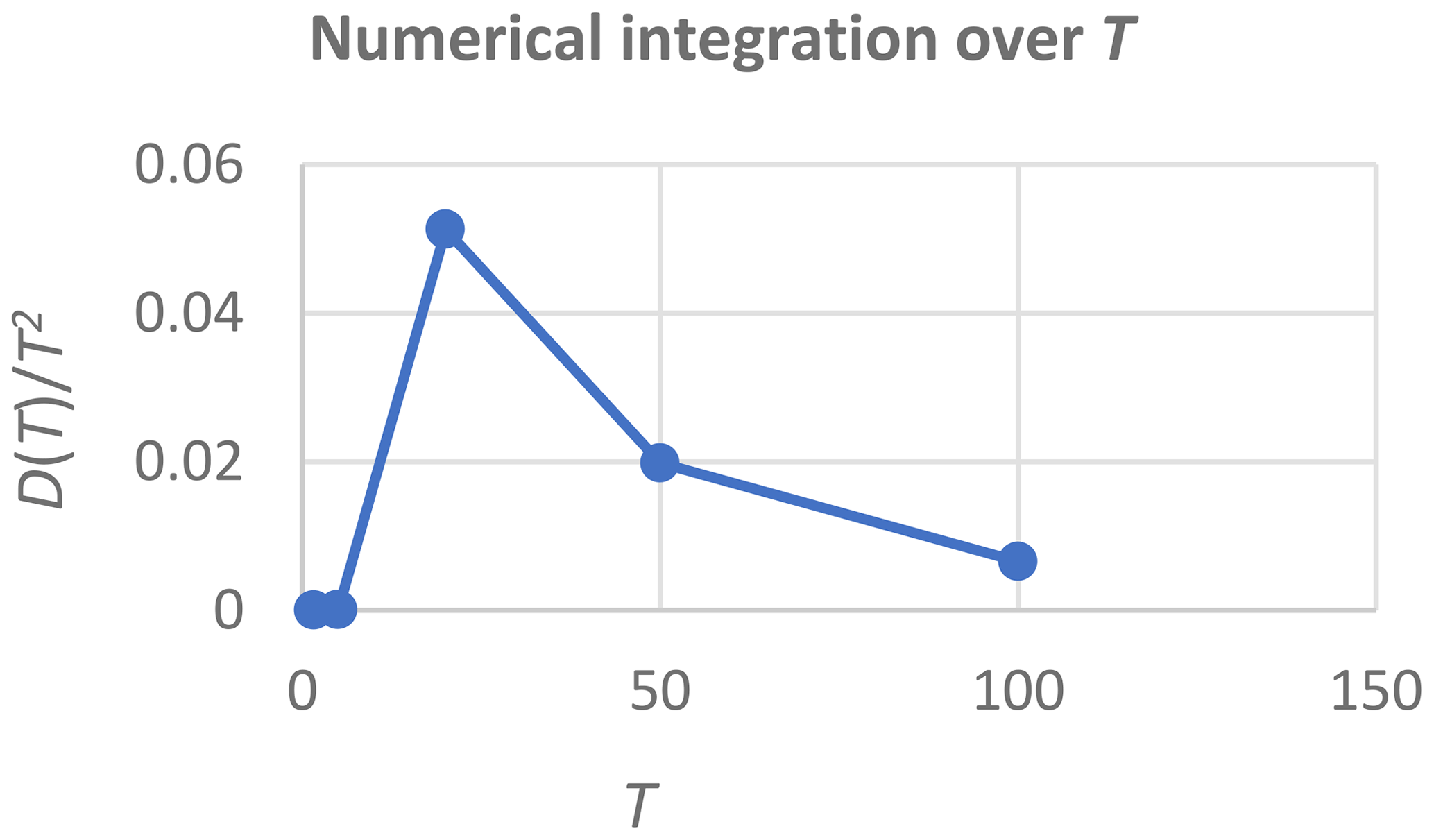
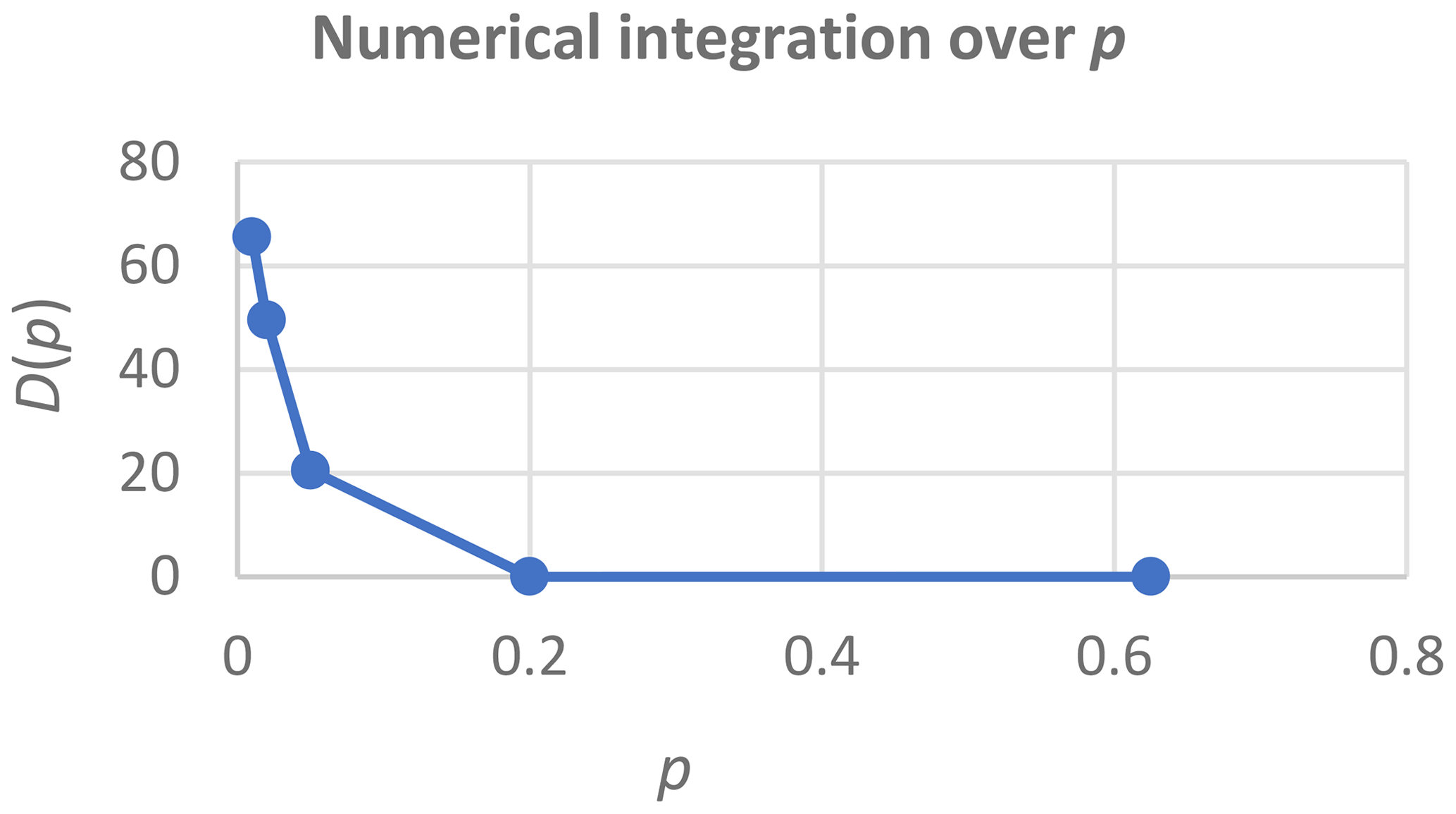
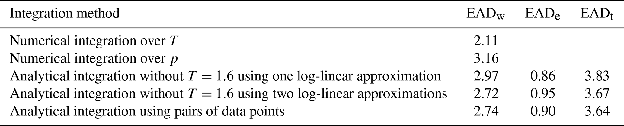
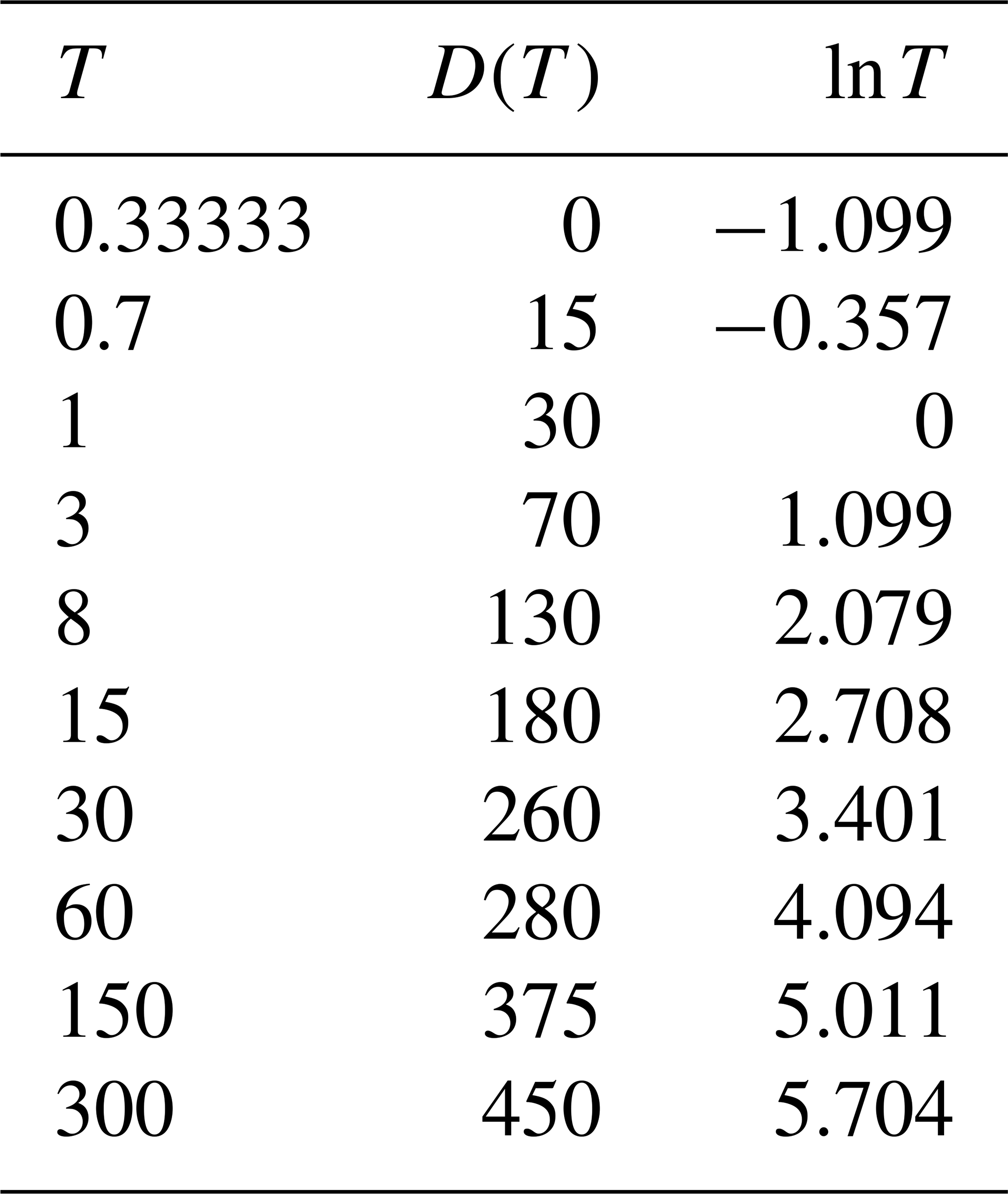
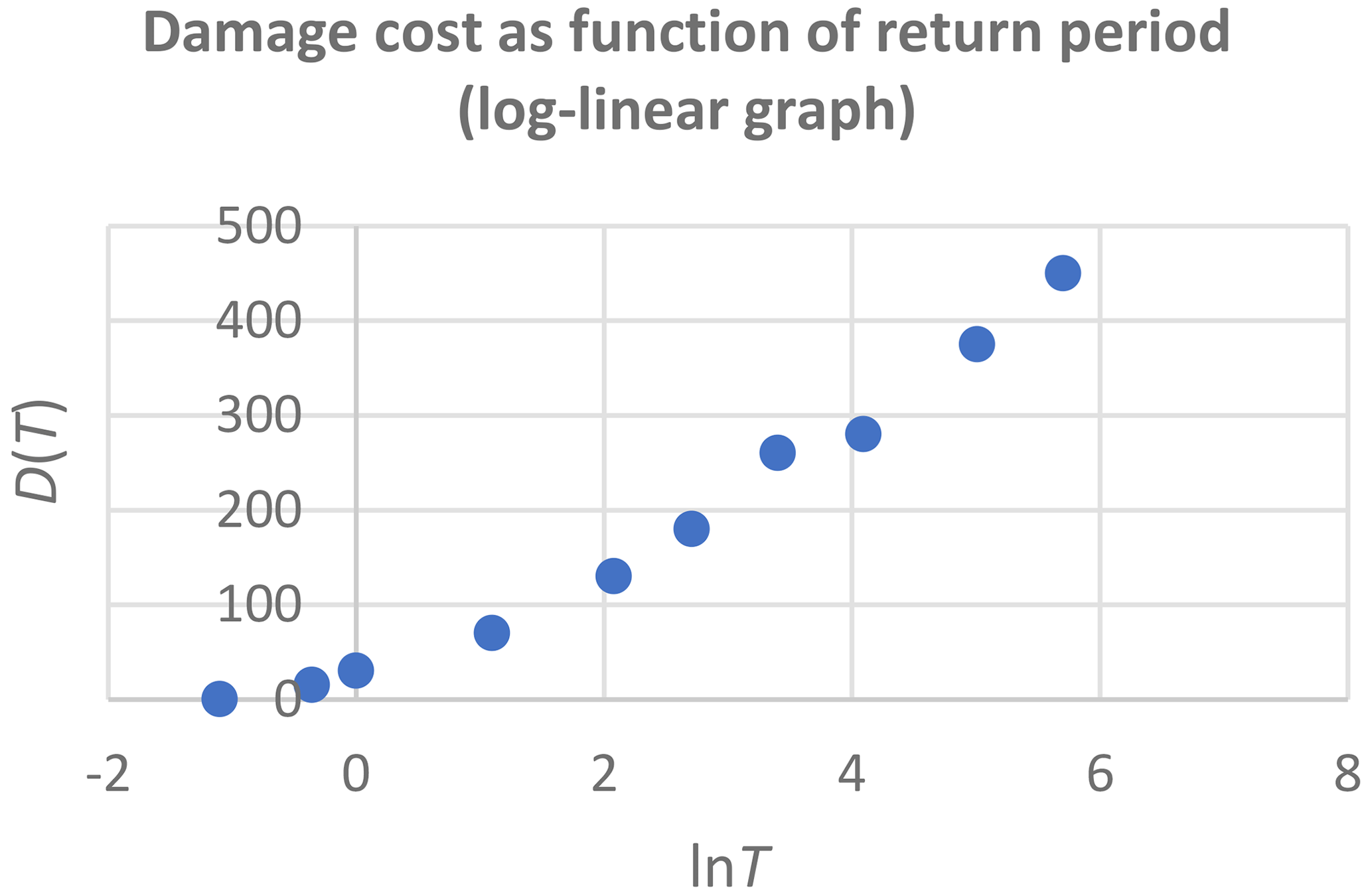
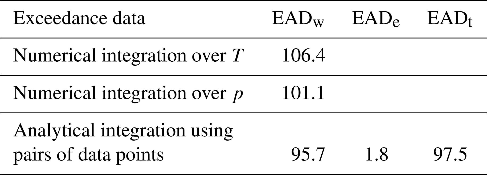
The sensitivity of expected annual damage, EAD, is analytically analysed by applying a log-linear relation between return periods and corresponding damages. It is found that the smallest return period for damage should be estimated as precisely as possible, that the percentage uncertainty in the damage estimate is transformed into the same percentage uncertainty in the EAD estimate, and that it is possible to extrapolate beyond the largest return period with corresponding damage assessment. The precision of the estimate of EAD is investigated in detail in the case of only few available data, and it is found that two different methods for numerical integration may result in strongly diverging results. By applying a piecewise log-linear damage function, it is shown that the log-linear model provides a trustworthy estimate of EAD, also in the case of few available data. Finally, the modifications needed in the special case of threshold exceedance data instead of annual maxima data are presented.

1 Introduction

In the future, large urban drainage structures in Denmark will be designed based on economic criteria instead of design based on a fixed return period (SVK, 2017). The societal value of the structure will be evaluated as the reduction in net present value of future damages less the net present value of investments and maintenance costs. Implicitly, it has been assumed that EAD (the expected annual damage) can be trustworthy determined. This, however, may strongly depend on the estimation method and the available data. Analytical estimation based on a log-linear relation between return period and corresponding damage (Olsen et al., 2015; Rosbjerg, 2017) is here further developed by introducing a stepwise integration. The method is evaluated by analysing two cases with, respectively, ample and sparse data availability. It is concluded that use of the analytical model is superior to straightforward numerical integration. Both annual maximum data and threshold exceedance data (known as peak over threshold series, POT, or partial duration series, PDS) are considered.

2 Theory

If the distribution function for the annual maximum X is denoted $F_X\left(x\right)=P\mathit{\{}X\le x\mathit{\}}$, the T-year event x_T is given by

$$\begin{array}{}\text{(1)}& F_X\left(x_T\right)=\mathrm{1}-{\displaystyle \frac{\mathrm{1}}{T_X}}=\mathrm{1}-p_X\end{array}$$

Consequently

$$\begin{array}{}\text{(2)}& x_T=F_X^{-\mathrm{1}}\left(\mathrm{1}-{\displaystyle \frac{\mathrm{1}}{T_X}}\right);T_X\ge \mathrm{1}\end{array}$$

The damage caused by the T_X year event is denoted by D_X(T_X) and the density function of X by $f_X\left(x\right)=\mathrm{d}{F}_X\left(x\right)/\mathrm{d}x$. Accordingly, EAD can be determined by

$$\begin{array}{}\text{(3)}& \text{EAD}={\int }_{\mathrm{0}}^{\mathrm{\infty }}{D}_X\left(x_T\right)f_X\left(x_T\right)\mathrm{d}{x}_T={\int }_{\mathrm{1}}^{\mathrm{\infty }}{\displaystyle \frac{D_X\left(T_X\right)}{T_X^{\mathrm{2}}}}\mathrm{d}{T}_X\end{array}$$

or

$$\begin{array}{}\text{(4)}& \text{EAD}={\int }_{\mathrm{0}}^{\mathrm{1}}{D}_p\left(p_X\right)\mathrm{d}{p}_X;D_p\left(p_X\right)=D_X\left({\displaystyle \frac{\mathrm{1}}{p_X}}\right)\end{array}$$

In practise, the integrations in Eqs. (3) and (4) are carried out inside the limits defined by available data.

In the case of threshold exceedance data with k exceedances per year in average and the distribution function for threshold exceedances Y denoted by G_Y(y), we get

$$\begin{array}{}\text{(5)}& G_Y\left(y_T\right)=\mathrm{1}-{\displaystyle \frac{\mathrm{1}}{k{T}_Y}}=\mathrm{1}-p_Y\end{array}$$

Consequently

$$\begin{array}{}\text{(6)}& y_T=G_Y^{-\mathrm{1}}\left(\mathrm{1}-{\displaystyle \frac{\mathrm{1}}{k{T}_Y}}\right);T_Y\ge {\displaystyle \frac{\mathrm{1}}{k}}\end{array}$$

Hereby EAD becomes

$$\begin{array}{}\text{(7)}& \text{EAD}={\int }_{\mathrm{1}/k}^{\mathrm{\infty }}{\displaystyle \frac{D_Y\left(T_Y\right)}{T_Y^{\mathrm{2}}}}\mathrm{d}{T}_Y\end{array}$$

or

$$\begin{array}{}\text{(8)}& \text{EAD}=k{\int }_{\mathrm{0}}^{\mathrm{1}}{D}_p\left(p_Y\right)\mathrm{d}{p}_Y;D_p\left(p_Y\right)=D_Y\left({\displaystyle \frac{\mathrm{1}}{k{p}_Y}}\right)\end{array}$$

Experience has shown and confirmed by the present analysis that a log-linear relation between return period and damage can be a good approximation.

$$\begin{array}{}\text{(9)}& D\left(T\right)=a\ln T+b\end{array}$$

where it may be assumed that the equation is valid also for $T->\mathrm{\infty }$. If D(T)=0 for T=T_s, then by integration from T_s to ∞ we get

$$\begin{array}{}\text{(10)}& \text{EAD}={\displaystyle \frac{a}{T_s}}\left(\mathrm{1}+\ln {\displaystyle \frac{T_s}{T_{\mathrm{0}}}}\right);T_{\mathrm{0}}=\exp \left(-{\displaystyle \frac{b}{a}}\right)\end{array}$$

Integration between two arbitrary return periods T_i and T_j greater than T_s leads to the EAD-contribution

$$\begin{array}{}\text{(11)}& \text{EAD}={\displaystyle \frac{a}{T_i}}\left(\mathrm{1}+\ln {\displaystyle \frac{T_i}{T_{\mathrm{0}}}}\right)-{\displaystyle \frac{a}{T_j}}\left(\mathrm{1}+\ln {\displaystyle \frac{T_j}{T_{\mathrm{0}}}}\right)\end{array}$$

If the log-linear relation is valid until T=T_c and then constant for $T_c<T<\mathrm{\infty }$, the contribution to EAD from the constant part is

$$\begin{array}{}\text{(12)}& \text{EAD}={\displaystyle \frac{a}{T_{\mathrm{0}}}}-{\displaystyle \frac{a}{T_c}}\left(\mathrm{1}+\ln {\displaystyle \frac{T_c}{T_{\mathrm{0}}}}\right)+{\displaystyle \frac{D\left(T_c\right)}{T_c}}\end{array}$$

3 Case A: Good data coverage

First, some initial sensitivity analyses are carried out based on annual maxima data with corresponding damage costs in a case with good data coverage, see Table 1. Implicitly, all costs are in mill. DKK. Case A refers to an idealised situation, where the data closely corresponds to the log-linear assumption.

Table 1 Case A – Damage cost as function of return period.

Inserting the regression parameters acquired from Fig. 1 into Eq. (10) results in the basic result shown in Table 2. The sensitivity of the result is investigated by varying input values one by one as indicated in Table 2. The numerical integrations are carried out based on Eq. (3).

Figure 1 Case A – Cost function in log-linear plotting.

Table 2 Case A – Sensitivity of EAD.

Some differences, but not substantial, are noticed between the obtained methods. An uncertainty of 10 % in the damage cost is seen to cause an uncertainty in EAD also of 10 %. Generally, the different results are of the same order of magnitude.

4 Case B: Sparse data coverage; numerical vs. analytical integration

Corresponding values obtained from Rambøll (2021) of annual maxima return periods and damage costs are shown in Table 3, and regression parameters obtained from a log-linear plot can be seen in Fig. 2. The limited number of cost estimates reflects the fact that it is quite labour intensive to estimate the costs. The figure reveals that the log-linear model provides a poor fit. However, by omitting the first data pair, which is justifiable since the resulting EAD value does not change at all when applying usual numerical integration, the log-linear fit is substantially improved. Having now only four data points justifies the characterization “sparse”.

Table 3 Case B – Damage cost as function of return period.

Figure 2 Case B – Cost function in log-linear potting.

In Figs. 3 and 4, the curves for numerical integration over, respectively, T and p are shown. Contrary to Case A, the integration results are here strongly differing. The area under the curve in Fig. 3 is found to be EAD =2.11, whereas the area under the curve in Fig. 4 is calculated to EAD =3.16 with no obvious explanation for the difference other than a strong non-linearity being present in both integrands. It makes no difference whether the first point in Table 3 is included or excluded.

Figure 3 Case B – Numerical integration over T (area below the curve).

Figure 4 Case B – Numerical integration over p (area below the curve).

The above results and corresponding results using the log-linear model combined with analytical integration are shown in Table 4. Suffix w means calculation without extrapolation, suffix e indicates calculation with extrapolation and suffix t the sum. Both one, two and pointwise log-linear approximations using Eq. (11) are applied.

Table 4 Case B – Numerical vs. analytical integration.

The results show that the log-linear model combined with analytical integration is generally applicable, also in the case of a sparse data set, where straightforward numerical integration appears inadequate. It is also seen that extrapolation can provide a significant supplement to the EAD value obtained by integration inside the interval covered by data.

5 Case C: Estimation of EAD with exceedance data

Here almost the same example as in case A is used, however slightly modified for T=1 and supplemented with two data pairs for T<1, see Table 5. The averages number of exceedances per year is k=3. The dataset is depicted in a log-linear graph in Fig. 5.

Table 5 Case C – Damage cost as function of return period.

Figure 5 Case C – Cost function in log-linear plotting.

The results of the different integration methods are shown in Table 6. As in case A, we see only moderate divergence between the different integration methods. Integration over T gives the largest value with integration over p being slightly below. However, in comparison with case A it is found that adding damage costs for return periods below T=1 implies a significant increase in the EAD estimate.

Table 6 Case C – Integration using exceedance data.

6 Conclusions

By analysing three cases, the following experience has been obtained.

Sensitivity

• It is important to know the return period for which damages get started, as frequent but small damages contribute significantly to EAD.

• Percentwise uncertainty in damage costs implies the same percentwise uncertainty in the estimate of EAD.

• The added supplement to EAD obtained by extrapolation can be significant.

Numerical integration

• Using numerical integration may result in diverging results when integrating over, respectively, T and p.

• In the case of a sparse data set, and for small values of T, the difference may be substantial.

Analytical integration

• Using a log-linear model combined with analytical integration is a flexible and convenient tool. A piecewise application down to data pairs is easily performed. The method provides trustworthy results and can be extrapolated to infinity, contrary to ordinary numerical integration.

References

Olsen, A. S., Zhou, Q, Linde, J. J., and Arnbjerg-Nielsen, K.: Comparing methods of calculating expected annual damage in urban pluvial flood risk assessments, Water, 7, 255–270, https://doi.org/10.3390/w7010255, 2015.
Rambøll: Manual for the application of Skrift 31, Miljøstyrelsen, https://www2.mst.dk/Udgiv/publikationer/2018/manual.pdf (last access: 21 January 2023), 2021 (in Danish).
Rosbjerg, D.: Optimal adaptation to extreme rainfalls in current and future climate, Water Resour. Res., 53, 535–543, https://doi.org/10.1002/2016WR019718, 2017.
SVK: Methods for determination of the service level for rainwater on the surface, IDA Spildevandskomitéen, https://spildevandskomiteen.dk/skrift-31/ (last access: 21 January 2023), 2017 (in Danish).
Download
Short summary
The paper provides a more precise and efficient method for calculation of the expected annual damage (EAD). Damage occurs when the current capacity is exceeded. An estimate of EAD is needed for the design of climate change adaptation measures based on economic optimisation, where future damages and maintenance costs are balanced against capital costs. The method is shown to be superior to estimation based on numerical integration, particularly in the case of sparse data availability.