A hybrid approach to enhance streamflow simulation in data-constrained Himalayan basins: combining the Glacio-hydrological Degree-day Model and recurrent neural networks

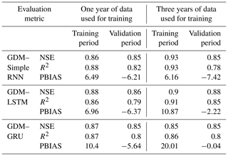
The Glacio-hydrological Degree-day Model (GDM) is a distributed model, but it is prone to uncertainties due to its conceptual nature, parameter estimation, and limited data in the Himalayan basins. To enhance accuracy without sacrificing interpretability, we propose a hybrid model approach that combines GDM with recurrent neural networks (RNNs), hereafter referred to as GDM–RNN. Three RNN types – a simple RNN model, a gated recurrent unit (GRU) model, and a long short-term memory (LSTM) model – are integrated with GDM. Rather than directly predicting streamflow, RNNs forecast GDM's residual errors. We assessed performance across different data availability scenarios, with promising results. Under limited-data conditions (1 year of data), GDM–RNN models (GDM–simple RNN, GDM–LSTM, and GDM–GRU) outperformed standalone GDM and machine learning models. Compared with GDM's respective Nash–Sutcliffe efficiency (NSE), R², and percent bias (PBIAS) values of 0.80, 0.63, and −4.78, the corresponding values for the GDM–simple RNN were 0.85, 0.82, and −6.21; for GDM–LSTM, they were 0.86, 0.79, and −6.37; and for GDM–GRU, they were 0.85, 0.8, and −5.64. Machine learning models yielded similar results, with the simple RNN at 0.81, 0.7, and −16.6; LSTM at 0.79, 0.65, and −21.42; and GRU at 0.82, 0.75, and −12.29, respectively. Our study highlights the potential of machine learning with respect to enhancing streamflow predictions in data-scarce Himalayan basins while preserving physical streamflow mechanisms.

1 Introduction

Hydrological models, classified as spatially distributed or lumped, differ in complexity and scope. While spatially distributed models cover diverse parameters across an area, lumped models use simpler relationships with fewer variables (Refsgaard and Knudsen, 1996). Physically based models aim for accuracy but may struggle with fine-scale features, often operating at larger scales with indirect parameter estimation (Beven, 2002). Despite their grounding in physical principles, they may not precisely represent all hydrological processes (Beven, 2002).

In high-mountain regions, like the Himalayas, distributed rainfall–runoff models face challenges due to the inadequate representation of snow and glacial processes. Glacio-hydrological models are crucial, but their effectiveness relies on data accessibility, with results influenced by the spatial and temporal resolutions (Réveillet et al., 2018). Despite the notion that increased data accessibility simplifies model construction, it often reveals the intricate nature of hydrological systems across diverse temporal and spatial scales (De Filippis et al., 2020).

Addressing inverse problems for calibrated hydrological models faces challenges like nonuniqueness and computational demands (Carrera et al., 2005). Uncertainties in hydrological models arise from observation accuracy, model variations, parameter distributions, estimation, and forcing variables (Dahlstrom, 2015).

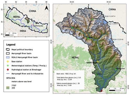
Figure 1 Map of Marsyangdi River basin, highlighting the river, tributaries, Bimalnagar hydrological station, Khudi Bazar base station, and meteorological stations. Publisher's remark: please note that the above figure contains disputed territories.

Figure 2 Schematic diagram of the GDM–RNN hybrid process.

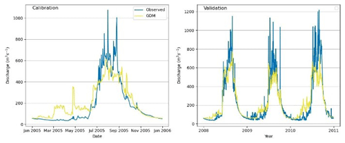
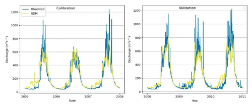
Figure 3 Observed vs. simulated discharges: the GDM model in the Marsyangdi River basin (1-year calibration and 3-year validation).

Machine learning algorithms aid parameter estimation, especially with abundant data (Solomatine, 2006). While physically derived models persist for comprehensive insights (Nearing et al., 2020), machine learning models complement them by addressing unpredictability or uncertainty (Solomatine, 2006). However, machine learning models lack interpretability as black-box models and may struggle in data-scarce regions like the Himalayan basin (Kayastha and Kayastha, 2019; Jia et al., 2020).

Debates on river discharge modeling focus on understanding physical processes vs. replicating observed values (Ji et al., 2021). An emerging solution combines both methods, using theory-based elements alongside data science to model residual errors. This approach constructs a residual error model to represent the theory-based model's discrepancies.

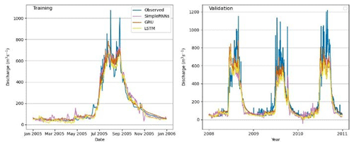
Figure 4 Observed vs. simulated discharges: different RNN models in the Marsyangdi River basin (1-year calibration and 3-year validation).

This research investigates the efficacy of recurrent neural networks (RNNs) with respect to modeling hydrological residual errors for improved streamflow predictions in data-constrained Himalayan basins. Specifically, the performance of different RNNs – simple RNN, a gated recurrent unit (GRU) model, and a long short-term memory (LSTM) model – is compared in contrast to a previous study's focus on LSTM alone (Cho and Kim, 2022). Simulations using the Glacio-hydrological Degree-day Model (GDM), simple RNN, GRU, and LSTM individually are also compared with proposed models (GDM–simple RNN, GDM–GRU, and GDM–LSTM).

2 Material and methods

2.1 Study area

The study area, Marsyangdi River basin in the Nepal Himalayas (Fig. 1), spans 4059 km², ranging from 355 to 7819 m a.s.l. (above sea level). About 13.3 % of the area is glacier-covered terrain, mainly between 4000 and 6500 m a.s.l. The basin experiences the Indian summer monsoon (June–September) and occasional westerly disturbances post-monsoon (October–January). Geographically, it features diverse terrain, primarily on the southern slopes of the Central Himalayas, influenced by the Annapurna Massif in the northwest.

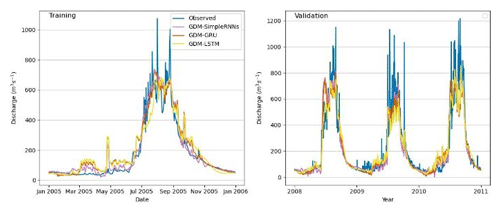
Figure 5 Observed vs. simulated discharges: different GDM–RNN models in the Marsyangdi River basin (1-year calibration and 3-year validation).

Figure 6 Observed vs. simulated discharges: the GDM model in the Marsyangdi River basin (3-year calibration and 3-year validation).

2.2 Glacio-hydrological Degree-day Model (GDM)

The Glacio-hydrological Degree-day Model (GDM, version 1.0) is a gridded hydrological model that evaluates the impact of various hydrological elements on river discharge (Kayastha and Kayastha, 2019). Operating daily, it incorporates snowmelt, glacier ice melt, rainfall, and baseflow runoff components. GDM utilizes a degree-day method for glacier ice melt and snowmelt, simplifying complex processes while minimizing data requirements.

Covering a 3×3 km gridded area, GDM assigns GlobeLand30 land categories to each grid and employs daily temperature and precipitation data from reference stations. It determines rain or snow in grids based on a threshold temperature. Daily ice melt and snowmelt in each grid consider debris-free and debris-covered ice, alongside glacierized and glacier-free regions.

The model computes surface runoff for each grid from precipitation, snowmelt, and ice melt. The cumulative surface runoff and baseflow from all grids contribute to the total discharge, directed to the outlet using a combined flow equation involving recession coefficients.

2.3 Recurrent neural networks (RNNs)

Recurrent neural networks (RNNs) are capable of capturing nonlinear connections in sequential data. They process input sequences element by element, utilizing a hidden state to retain information about past inputs, allowing predictions based on historical context. RNNs are suitable for regression problems, predicting continuous outputs from input sequences. Training involves employing regression loss functions like mean-squared error or mean absolute error (Heaton et al., 2018).

RNN components include an input layer, recurrent unit, hidden state, activation function, output layer, loss function, and optimization algorithm. Hyperparameters in RNNs control network behavior, impacting the capacity, convergence speed, overfitting, sequence length, dropout, layers, activation function, optimization algorithm, learning rate decay, and early stopping (Heaton et al., 2018). Types of RNNs include the simple RNN, LSTM, and GRU models. Simple RNN models possess limited memory for short-term sequences (Bengio et al., 1994). LSTM introduces memory cells and gates controlling data flow, enabling long-term memory retention (Hochreiter and Schmidhuber, 1997). GRU combines input and forget gates into an update gate, requiring fewer parameters than LSTM, but offering similar performance (Cho et al., 2014).

2.4 The GDM–RNN hybrid approach

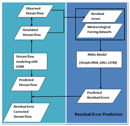
The study introduces a GDM–RNN hybrid approach that aims to improve streamflow prediction by integrating GDM's physical constraints. This approach utilizes RNNs (simple RNN, GRU, and LSTM models) to forecast residual errors between observed and GDM-simulated inflows based on meteorological inputs. Given the complexity of quantifying these errors, the assumption is made that they exhibit identifiable patterns. The RNNs operate independently after GDM simulation to optimize error prediction without disturbing the physical constraints. Figure 2 outlines this hybrid process, involving the generation of simulated streamflow data via GDM, computation of residual errors, optimization, training of RNN models using these errors and meteorological data, projection of future errors, and application of these predictions to enhance GDM simulations. This approach intends to improve traditional GDM simulations by accounting for predictive discrepancies originating from various uncertainties.

2.5 Input data

Daily air temperature, rainfall, and river flow data are obtained from the Department of Hydrology and Meteorology (DHM). Temperature and rainfall data from Khudi Bazar and Chame stations are used for the GDM, while Bimalnagar outlet station's discharge data validated the study. RNNs were trained using the climatic stations' temperature, rainfall data, and discharge data from Bimalnagar. The GDM relied on elevation information from ASTER Global Digital Elevation Model Version 2 and land cover data from the GlobeLand30 dataset. Six land classes were identified and modified for uniform rainfall–runoff factors. Glacier identification was based on the International Centre for Integrated Mountain Development (ICIMOD) glacier inventory of shapefiles from 2010.

2.6 Experimental designs

The study employed seven models: GDM, GDM–LSTM, LSTM, GDM–GRU, GRU, GDM–simple RNN, and simple RNN. Each GDM model variant combined with RNNs aimed to predict residual errors. RNNs were used for river discharge simulation and performance comparisons with GDM models and GDM–RNN hybrids. Two datasets were used for calibration/training: a 1-year dataset and a 3-year dataset. GDM and RNNs were calibrated/trained using 2005 data and validated with 2008–2010 data. The GDM coupled with RNNs utilized 2005 data for calibration, predicting residual errors (2008–2010). Similarly, the experiment was repeated using data from 2005 to 2007 for calibration and training purposes. The models were then validated using 2008–2010 data. Discharge simulations by GDM (2008–2010) were corrected using predicted residual errors from RNNs, and the results were validated using observed discharge data (2008–2010).

The streamflow forecasts of various models were assessed utilizing three widely utilized measures for hydrological model evaluation: percent bias (PBIAS), Nash–Sutcliffe efficiency (NSE), and R² (Moriasi et al., 2015).

3 Results and discussions

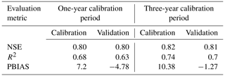
In the Glacio-hydrological Degree-day Model (GDM) calibration, adjustments are made in positive degree-day factors, snow and rain coefficients, and the recession coefficient. Parameters are calibrated for 1-year and 3-year periods using observed streamflow data from the Marsyangdi River basin. The model closely replicated observed data for both periods, with slightly better performance in the 3-year calibration (Fig. 3). Although the model generally matched observed outflow, it tended to overestimate during low-flow periods due to challenges with respect to accurately depicting precipitation distribution, especially at higher altitudes (Immerzeel et al., 2015; Bocchiola et al., 2011; Barry, 2012). Evaluation metrics (NSE, R², and PBIAS) indicated a satisfactory fit but showed some bias, with the model overestimating in the calibration and underestimating in the validation (Table 1).

Table 1 The NSE, R², and PBIAS metrics during the GDM model calibration and validation periods.

Table 2 The NSE, R², and PBIAS metrics for different RNNs used in the RNN-only approach.

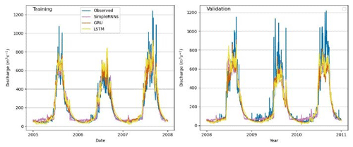
Figure 7 Observed vs. simulated discharges: different RNN models in the Marsyangdi River basin (3-year calibration and 3-year validation).

In this study, RNN models (simple RNN, LSTM, and GRU) are trained using 1-year and 3-year datasets, employing diverse training parameters including network architecture, activation functions, optimization algorithms, loss functions, and training schedules. Models preprocessed input data through normalization and utilized Adam optimization with a mean absolute error loss function. The number of hidden layers and neurons varied among models; all had 4 input units and 1 output unit, with GRU and LSTM using 128 neurons in a hidden layer, while simple RNN employed 32. The learning rate is constant at 0.01 but had varied schedules. In this study, the parameters of the RNN models are selected using the grid search technique.

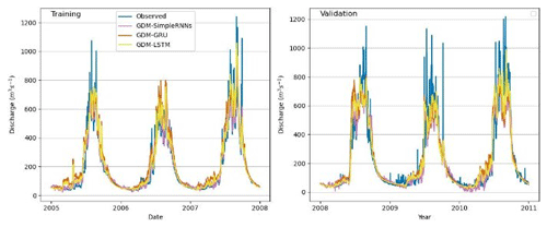
Figure 8 Observed vs. simulated discharges: different GDM–RNN models in the Marsyangdi River basin (3-year calibration)

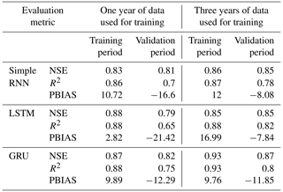
Analysis shows superior performance for RNNs with 3 years of data compared with those with 1 year of data. LSTM and GRU exhibited better simulation of river discharge patterns than simple RNN models, especially with extensive training data, indicating a greater capacity to learn past streamflow behaviors. However, smaller datasets yielded only satisfactory results, suggesting the suitability of process-based models like GDM. Evaluation metrics demonstrated GRU's superior performance across NSE, R², and PBIAS for both 1-year and 3-year validation periods, while LSTM excelled slightly with respect to the R² value for the 3-year period. Simple RNN consistently showed the poorest performance (Table 2).

Positive PBIAS during training suggests model overestimation, potentially due to overfitting, whereas negative PBIAS during validation implies underestimation, indicating an inability to capture relevant data aspects. Despite better performance on training data, the emphasis lies on a model's ability to generalize to new data, highlighting the significance of validation results. Overall, GRU showcased superior performance in key metrics across different training periods, with LSTM showing competitive results in specific aspects.

Hybrid modeling combined GDM and three RNN variants (simple RNN, LSTM, and GRU) to predict GDM residual errors. The hybrid approach split into simulating streamflow using GDM parameters and training RNNs to predict errors (Table 3). All RNNs featured a single hidden layer with 64–254 neurons, tanh activation in the hidden layer, and linear activation in the output layer, using Glorot uniform kernel initialization. Input data normalization is applied. Key hyperparameters varied, including dropout rates (0.2–0.6), Adam optimization, batch size equivalent to the entire training set, a sequence length of 365 d, and a fixed learning rate of 0.01. Learning rate schedules varied or were absent, employing strategies like exponential or inverse time-based decay. The grid search technique is used to select the best-performing parameters.

Table 3 The NSE, R², and PBIAS metrics for different GDM–RNN models.

The integration of GDM and RNN models (GDM–RNN) outperforms the sole use of RNNs for streamflow prediction. GDM–RNN provides more stable predictions, using residual discrepancies as objectives, while RNNs directly predict streamflow. This disparity in objectives impacts the model forecasts, potentially causing greater systematic discrepancies in RNNs due to streamflow variability.

GDM–RNN (Figs. 4–8) simulation aligns better with physical discharge patterns, addressing issues like negative discharge seen in simple RNN (Fig. 4). It particularly excels with 1 year of observed discharge data, significantly improving simulations compared with RNNs with the same training data. GDM–RNN enhances GDM's streamflow prediction by reducing uncertainties and effectively resolves high-discharge issues in the pre-monsoon season. During the monsoon, GDM–RNN (Fig. 8) closely matches observed discharge compared to GDM (Fig. 6) simulations.

4 Conclusions

Our study highlights the effectiveness of utilizing LSTM, GRU, and simple RNN machine learning techniques to improve streamflow forecasting within the GDM model in the Marsyangdi River basin, Nepal. The amalgamation of GDM and RNNs significantly enhances predictive accuracy, notably in terms of the NSE and coefficient of determination, while displaying comparable performance in PBIAS to GDM alone. The limitations of RNNs, particularly with respect to handling high-variability datasets, contribute to disparities in PBIAS measures compared with GDM. Furthermore, while GDM shows consistent performance across varying calibration dataset sizes, RNNs benefit significantly from increased training data. Notably, the GDM–RNN model displays superior adaptability with limited calibration and training data, showing notable improvements with increased dataset sizes. GRU and LSTM outperform simple RNN due to their capacity to handle long-term dependencies, both in standalone RNN usage and in hybrid combinations.

Evaluation in a single basin with limited data showcases the robustness of GDM–RNN and the potential of RNN implementation. Expanding validation with 3 years of data or across different basins would enhance its reliability. While comparing two datasets demonstrated promising results, examining additional data could further strengthen our approach.