the Creative Commons Attribution 4.0 License.
the Creative Commons Attribution 4.0 License.
 | 19 Apr 2024
Satellite and UAV derived seasonal vegetative roughness estimation for flood analysis
Andre Araujo Fortes
Masakazu Hashimoto
Keiko Udo
Ken Ichikawa
One of the purposes of river management is the disaster protection of the nearby population. The effect of riparian vegetation on hydraulic resistance and conveyance capacity makes it a vital parameter for this purpose. With remote sensing techniques, vegetation information can be estimated. This paper's objective is to combine UAV and satellite imagery to obtain vegetation parameters with moderate resolution for hydraulic modeling, and to assess the seasonal effect of the vegetation on the Manning coefficient. Typhoon Hagibis was simulated with a 2D hydraulic model with a dynamic vegetative roughness estimation routine. Results demonstrate that this method achieved less error than the traditional static roughness value method of hydraulic modeling. The seasonal effect of the vegetation on the roughness was shown by a relationship between the percentage of vegetation cover and the average Manning in the stretch.
- Article
(2300 KB) - Full-text XML
- BibTeX
- EndNote


On 12 October 2019, typhoon Hagibis hit Japan causing extreme rainfall and flooding several rivers across the territory (Kazama et al., 2021). River management is tasked to provide the safety of nearby populations from floods, thus accurate predictions of these events and mitigation measures must be made. Hydraulic models are used to provide information on flood risk and vulnerability, but many input data are needed, such as topography, flow data, and the Manning roughness coefficient, to provide accurate results (Bates, 2004).
Vegetation is the dominant factor in determining the roughness value (Ebrahimi et al., 2008), and their physical parameters are the primary determinants (Nikora et al., 2008). Studies show that plant density impacts the roughness while the vegetation is emergent (Aberle and Järvelä, 2013), and the ratio of the flow depth to the canopy height describes the roughness in the submerged state (Nikora et al., 2008). A good descriptor of plant density is the leaf area index (LAI) (Jalonen et al., 2013), which is defined as the total one-sided leaf area over ground unit area.
With vegetation mostly located in the floodplains, it is a common practice to adopt constant roughness values for channel and floodplains. This practice requires a time-consuming process of trial and error to obtain accurate results. According to Ebrahimi et al. (2008), the adoption of a dynamic Manning value varying with changes in flow and vegetation conditions can obtain better results than static Manning approaches. In addition, with seasonal changes in the vegetation parameters, variations in the hydraulic resistance also occur. Therefore, studies that combine the application of vegetation parameters on hydraulic models in real scenarios are very important.
With advancements in remote sensing techniques, obtaining vegetation physical parameters has become cheaper and less time-consuming (Fortes et al., 2022). The use of unmanned aerial vehicles (UAVs) equipped with cameras eased the identification and extraction of features such as vegetation height and their variation with the passing of seasons (van Iersel et al., 2018). Satellites have the advantage of more temporal frequency, covering a larger area, and with emission of more spectral bands, many indices can be obtained, although with less resolution than UAVs. Vegetation parameters can also be obtained from these sources (Gokool et al., 2022).
Besides vegetation parameters, new technologies have allowed the acquisition of high-resolution spatially distributed water levels, such as the ICESat-2 satellite mission (Coppo Frias et al., 2023) and UAVs equipped with radar altimetry (Jiang et al., 2020), which can be useful in hydraulic modeling for calibration and validation.
The objective of this study is to combine UAV and satellite imagery to obtain LAI and vegetation height with moderate resolution for hydraulic modeling, with dynamic vegetative roughness calculation, and to assess the seasonal effect of the vegetation on the roughness parameter.
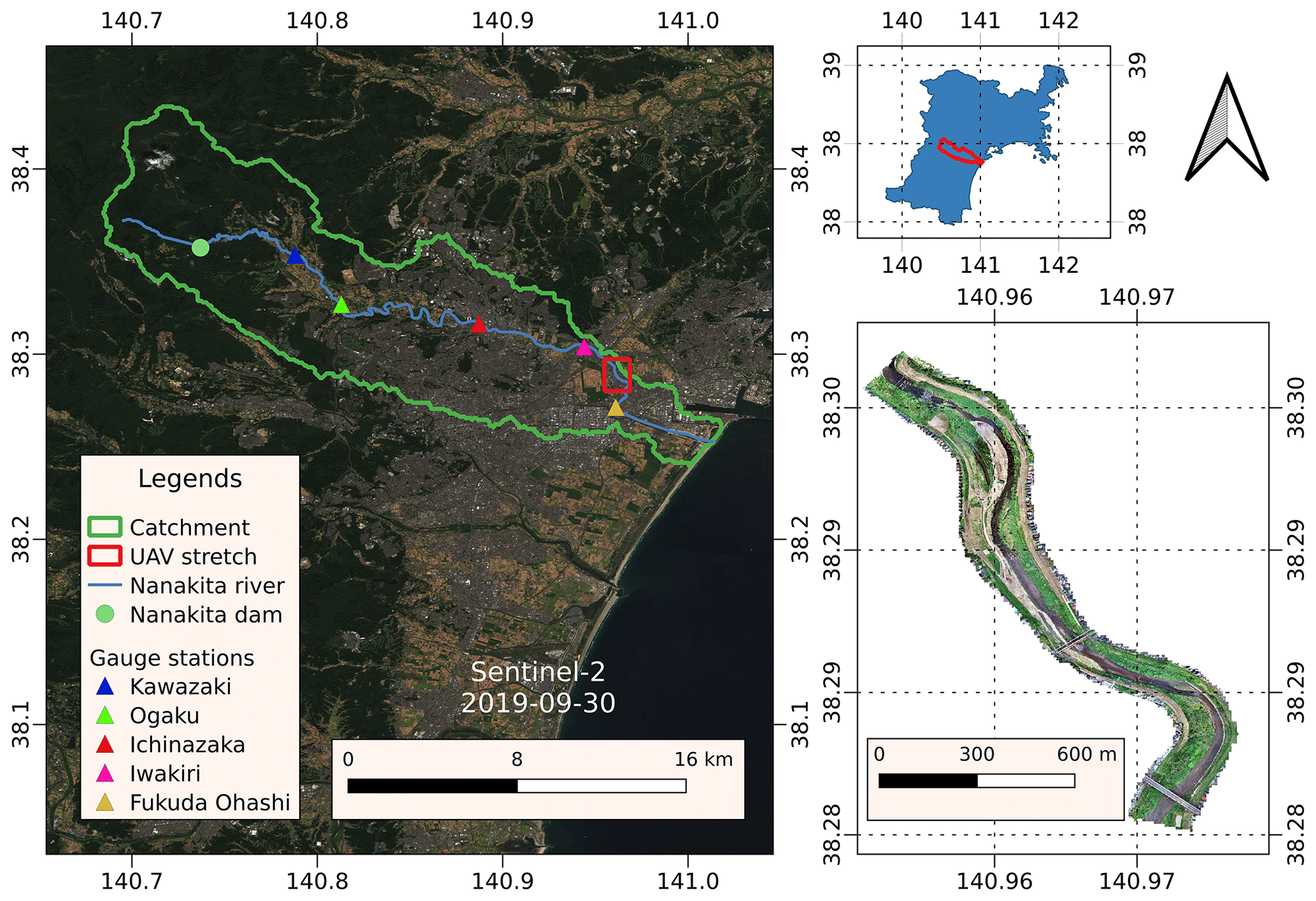
Figure 1Study area, showing the location of the catchment and the location of the 2 km stretch, where the hydraulic model was applied.
The hydraulic model was applied in a 2 km stretch of the Nanakita river, in the Miyagi prefecture of Japan. The river has 45 km of total length and, catchment area of 229 km2. The mean annual discharge is 10 m3 s−1 and the 100-year return period discharge is 1650 m3 s−1 (Viet et al., 2006). According to Pilailar et al. (2003), the bed slope of Nanakita river is about 0.0016 in the upstream and 0.0003 in the downstream part of the river. Rivers in Japan are classified as class A or class B rivers, depending on their size. Class A rivers are managed by the national government and class B rivers, like Nanakita river, are managed by the local prefectures. UAV flights took place in the 2 km stretch in September 2019, and then monthly from April 2020 to March 2021. Figure 1 shows the catchment location and the location of the 2 km stretch of the river.
The vegetation in the stretch is mostly comprised of shrubs and tall grass species. The predominant population is Pueraria montana var. Lobata (Kudzu), Miscanthus sinensis, Phragmites australis, and Solidago canadensis.
During typhoon Hagibis, no overtopping of the flood control structures occurred in the 2 km stretch.
To recreate the typhoon Hagibis flood event in the stretch, three 2D-hydraulic simulations were performed. One simulation using constant Manning values, from here referred to as Static Manning Simulation (SMS), and two simulations with dynamic Manning calculation. In the dynamic set, one simulation calculated the Manning value only in submerged vegetation scenario, with the method used in Fortes et al. (2022), from here referred to as Partial Dynamic Manning Simulation (PDMS), and the other calculated the Manning value for submerged and emergent vegetation scenarios, referred as Full Dynamic Manning Simulation (FDMS).
After the event recreation, the effect of seasonal variation of the vegetation on Manning was assessed by simulating the same event with vegetation conditions in each season. The UAV observation and sentinel-2 images from May 2020, November 2020, and January 2021 were used to represent spring, autumn, and winter, respectively. The recreation of the event used the observation from September 2019, representing the summer season. To perform the seasonal assessment, the FDMS model was used. The input data for the hydraulic simulation of each season was the same, differing only in the LAI and vegetation height values and distribution.
The upstream discharge used in the hydraulic models was obtained from Fortes et al. (2022), using a hydrologic model, covered in Sect. 3.1. Section 3.2 covers the hydraulic model used for the SMS and the topography used. The vegetative Manning algorithms are introduced in Sect. 3.3, and Sect. 3.4 explains the method to obtain the vegetation parameters.
3.1 Hydrologic simulation
The input discharge was obtained by running a hydrologic model, the Rainfall-Runoff Inundation (RRI) model, which is capable of simulating both rainfall-runoff and inundation phenomena (Sayama et al., 2012). It uses continuity and momentum equations as governing equations.
The input data was the catchment digital elevation model (DEM), obtained from MERIT Hydro (Yamazaki et al., 2019) with 90 m resolution, rainfall data from the radar/raingauge-analyzed (RA) precipitation (Ishizaki and Matsuyama, 2018) from 12–14 October 2019, land cover obtained from MLIT National Land Data Information (2014) with 100 m resolution and the Manning data, which was set 0.04 in river cells and in the slope cells, 0.5 for vegetation, 0.3 for urban areas and 0.04 in water bodies.
The outputs are the inundation map, water level, and discharge. The validation was obtained by comparing the simulated and observed water depth at the five water level gauge stations shown in Fig. 1.
3.2 Hydraulic model
A 2D hydraulic model was used for the event recreation in the stretch (Hashimoto et al., 2018). The model uses continuity and momentum equations as governing equations. The model's input data are the topography, the upstream discharge, and the Manning values. The outputs are the inundation and water level. The hydraulic model inputs as boundary conditions the outlet cells and their slope.
The computational domain for the hydraulic model was the 2 km UAV observed stretch of the river, shown in Fig. 1. The DEM used as topography input in all hydraulic simulations was constructed from 21 cross-sections provided by Miyagi prefecture. The final resolution of the DEM was 10 m. The Manning setting for the SMS was 0.022 for the channel and 0.038 for floodplains, as recommended by Miyagi prefecture. To distinguish channel and floodplain, a simulation using the average annual discharge of the river was performed. This method was chosen rather than making this classification from the topography because setting a height threshold to separate river and floodplain areas would not consider the slope progression of the river. Using the mean annual discharge was preferred because pre-calibrated roughness values for the river channel were available and could be used to observe where the water surface would accommodate in the stretch.
Outlet cells were selected as the boundary condition. The outlet discharge was calculated with Manning equation, and the slope was set as 0.0002, which is close to the average slope of the lower reaches of the river.
All models were validated by comparing simulated and observed water level profiles in 5 sections. The height was obtained by observation of photos taken during the event, the height of objects in the photographs was used to estimate the height difference between the top of the embankments and the watermarks.
3.3 Dynamic Manning routine
While the FDMS introduces the Manning calculation in the emergent state of the floodplain vegetation, the PDMS was performed using the algorithm developed by Fortes et al. (2022), which used only the submerged state to calculate the Manning values cellwise, blocking the water flow at the vegetated cells while in emergent state. The reason for considering using the PDMS is due to the coefficients needed by the FDMS, which are not always available.
3.3.1 Emergent vegetation state
The vegetation LAI was used for this state. The Darcy-Weisbach friction factor at each cell was calculated from Eq. (1), proposed by Järvelä (2004).
where f is the friction factor, CDx is the vegetation drag coefficient, “LAI” is the LAI value in the cell, x is a species-specific constant, u is the flow velocity, ux is the minimum velocity used to find the x value, h is the water depth, and hveg is the vegetation height. The CDx, x, and ux were obtained from Aberle and Järvelä (2013).
The friction factor was then converted to the Manning coefficient using Eq. (2), from Box et al. (2021).
where g is the gravitational acceleration.
3.3.2 Submerged vegetation state
As explained in Fortes et al. (2022), for submerged state, the Manning coefficient was calculated by its relationship with the degree of submergence of the vegetation. The data was obtained from Japan Institute of country-ology and engineering (2002) and with regression analysis an exponential formula was obtained with a coefficient of determination (R2) of 0.87, shown in Eq. (3).
where hveg is the height of the vegetation and hwater is the water depth.
3.4 Vegetation parameters
A k-means clustering algorithm was used in a sample of the UAV image based on the RGB values, then visual supervision was applied to obtain the vegetated cells and a multi-layer Perceptron (MLP) algorithm was trained, and then used to predict the vegetated cells in the entire stretch.
The vegetation height was obtained by normalizing the digital surface model (DSM) values, which comprises both ground and above objects elevation, with the DEM values in the vegetated cells. A more detailed explanation of the method applied for the vegetation identification and height calculation is found in Fortes et al. (2022).
3.4.1 Leaf area index
The leaf area index was obtained by downscaling the MODIS LAI product from 500 to 10 m resolution using machine learning (ML), like in Gokool et al. (2022).
An MLP regressor model was trained using NDVI and EVI from MODIS as input variables and MODIS LAI as the target variable in the entire Tohoku region of Japan. To represent the summer seasons, MODIS images dating from 1 July 2020 to 30 September 2020 were averaged, then the model was trained. Afterward, Sentinel-2 NDVI and EVI with 10 m resolution from 30 September 2019 in the study area were used in the trained model to obtain the LAI values over the catchment. The LAI values were then confined to the vegetated cells in the UAV observation.
Different ML models were trained for each season with the same method, using the averaged MODIS values from 1 January to 31 March 2020 (winter), 1 April to 30 June 2020 (spring), and 1 October to 31 December 2020 (autumn). Sentinel-2 images for each season were used to predict their respective LAI values and distribution in the stretch.
4.1 Vegetation conditions
The vegetation location was successfully obtained, with the MLP model achieving an accuracy of 0.99 for summer and spring and 0.96 for autumn and winter (Fortes et al., 2022).
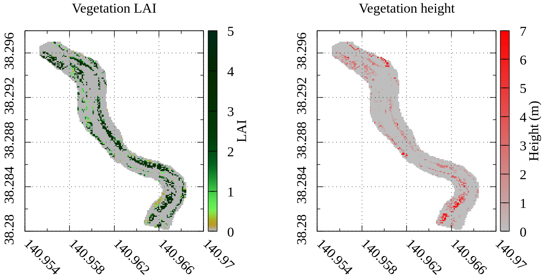
Figure 2LAI and vegetation height in the stretch from the observation of September 2019 (summer season).
The total vegetated area in September 2019 was 82 800 m2, representing about 18 % of the total area of the stretch. The height of the vegetation was 1.7 m in average and the LAI was 2.43 in average. Figure 2 shows the estimated vegetation height and LAI in the stretch in the summer period, from the observations from September 2019.
4.2 Hydrologic simulation
As shown in Fortes et al. (2022), the RRI simulation could produce accurate results, with simulated water depth similar to the observed. Nash-Sutcliffe coefficient at each of the stations was −0.37 in Kawazaki, 0.77 in Ogaku, 0.88 in Ichinazaka, 0.73 in Iwakiri, and 0.62 in Fukuda Ohashi. Since most values ranged from 0.62 to 0.88, reaching values close to 1, the simulation was considered accurate, and the discharge obtained in the upstream section of the stretch was used in the hydraulic model. The peak discharge at the outlet was about 1250 m3 s−1, lower than the peak discharge of a 100-year return period flood event. In the stretch upstream, it was about 1050 m3 s−1.
4.3 Hydraulic simulations
The recreation of the typhoon event has shown a fair result when comparing simulated and observed water levels. The RMSE calculated for each simulation was 0.141 for SMS, 0.189 for PDMS, and 0.137 for FDMS. Figure 3 shows the peak water profile of the three simulations and the observed points.
The SMS and FDMS achieved the best results, closer to the observed water level. On the other hand, the PDMS achieved a higher water level, presenting an overestimation of the inundation. This happened due to the blockage of water flow in the emergent vegetation state. With Manning being dynamically calculated for both vegetation states, the FDMS presented a similar result when compared with the SMS, suggesting that the applied Manning algorithm is a valid substitute for calibrated static Manning values. The FDMS achieved the lowest RMSE, which agrees with the conclusions of Ebrahimi et al. (2008). This is important because the FDMS model does not require much calibration in terms of Manning value, with calibration being necessary only for the non-vegetated cells.
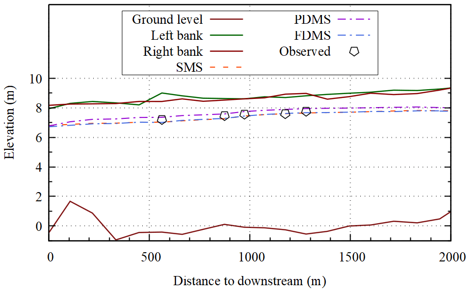
Figure 3Longitudinal view of simulated water level and observed water level at five sections during peak inundation.
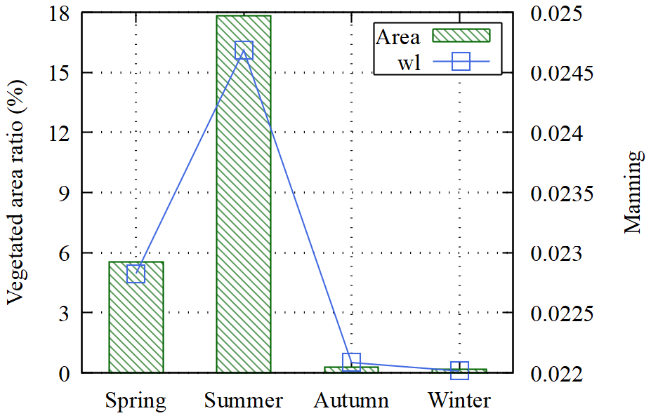
The seasonal changes of the vegetation conditions were as expected. Due to the lack of foliage, the vegetated area drastically reduced during the autumn and winter seasons. The peak vegetated area was in summer, followed by spring. The Manning values in the peak water level of each simulation were averaged for the entire terrain and compared with the ratio of the vegetated area over the entire stretch area.
Figure 4 shows the vegetated area in each season and the peak average Manning value. It clearly shows that the average Manning values strongly relate to the percentage of vegetated area in the stretch. Regarding the effect of the vegetation on the water level profile of each season, with the highest Manning, value, presented the highest water level profile of all seasons. The difference in water level between spring, autumn, and winter was not very perceptible. The highest difference in the water level profiles was between summer and winter, with 27.1 centimeters on average, and the lowest was between summer and spring, with 26.4 centimeters.
Machine learning proved to be an effective tool to acquire remote sensing vegetation data. The typhoon event could be accurately reconstructed in the study area. The FDMS presented the lowest RMSE value of 0.137, with a water level profile similar to the one produced by the SMS. This means that the Manning calculation algorithm worked well and was a good substitute for the static Manning of 0.038. The FDMS presented the advantage of requiring less calibration to achieve accurate results. Since the PDMS did not consider water flow in the emergent vegetation, it presented an overestimation of the inundation, being less applicable. The results show an advance in considering vegetation parameters to calculate Manning at a pixel level, but the models need to be tested in more rivers to fully validate the Manning algorithm.
The seasonal effect of the vegetation was demonstrated when the average Manning in the stretch in the peak was compared to the ratio of vegetated area, which demonstrated a strong relationship.
Due to copyright restrictions, the code for the 2D flow model cannot be shared without the permission of the developers. The part for the vegetative roughness calculation can be shared upon request.
The data can be available upon request.
AAF was responsible for Conceptualization, Investigation, Methodology, Software, Formal analysis, Visualization, and Writing – original draft preparation. The co-authors contributed as follows: MH participated in Methodology, Software, Data curation, Supervision, Validation, and Writing – review & editing, KU participated in Methodology, Validation, Supervision, Project administration, and Writing – review & editing, KI participated in Data curation, Resources, and Writing – review & editing.
The contact author has declared that none of the authors has any competing interests.
Publisher's note: Copernicus Publications remains neutral with regard to jurisdictional claims made in the text, published maps, institutional affiliations, or any other geographical representation in this paper. While Copernicus Publications makes every effort to include appropriate place names, the final responsibility lies with the authors.
This article is part of the special issue “ICFM9 – River Basin Disaster Resilience and Sustainability by All”. It is a result of The 9th International Conference on Flood Management, Tsukuba, Japan, 18–22 February 2023.
This paper was edited by Daisuke Harada and reviewed by two anonymous referees.
Aberle, J. and Järvelä, J.: Flow resistance of emergent rigid and flexible floodplain vegetation, J. Hydraul. Res., 51, 33–45, https://doi.org/10.1080/00221686.2012.754795, 2013.
Bates, P.: Remote sensing and flood inundation modelling, Hydrol. Process., 18, 2593–2597, https://doi.org/10.1002/hyp.5649, 2004.
Box, W., Järvelä, J., and Västilä, K.: Flow resistance of floodplain vegetation mixtures for modelling river flows, J. Hydrol., 601, 126593–126604, https://doi.org/10.1016/J.JHYDROL.2021.126593, 2021.
Coppo Frias, M., Liu, S., Mo, X., Nielsen, K., Ranndal, H., Jiang, L., Ma, J., and Bauer-Gottwein, P.: River hydraulic modeling with ICESat-2 land and water surface elevation, Hydrol. Earth Syst. Sci., 27, 1011–1032, https://doi.org/10.5194/hess-27-1011-2023, 2023.
Ebrahimi, N. G., Fathi-Moghadam, M., Kashefipour, S. M., Saneie, M., and Ebrahimi, K.: Effects of Flow and Vegetation States on River Roughness Coefficients, J. Appl. Sci., 8, 2118–2123, 2008.
Fortes, A., Hashimoto, M., Udo, K., Ichikawa, K., and Sato, S.: Dynamic Roughness Modeling of Seasonal Vegetation Effect: Case Study of the Nanakita River, Water, 14, 3649–3667, 2022.
Gokool, S., Kunz, R. P., and Toucher, M.: Deriving moderate spatial resolution leaf area index estimates from coarser spatial resolution satellite products, Remote Sens. Appl.-Soc. Environ., 26, 100746–100758, https://doi.org/10.1016/j.rsase.2022.100743, 2022.
Hashimoto, M., Yoneyama, N., Kawaike, K., Deguchi, T., Hossain, M. A., and Nakagawa, H.: Flood and Substance Transportation Analysis Using Satellite Elevation Data: A Case Study in Dhaka City, Bangladesh, J. Disaster Res., 13, 967–977, https://doi.org/10.20965/jdr.2018.p0967, 2018.
Ishizaki, H. and Matsuyama, H.: Distribution of the Annual Precipitation Ratio of Radar/Raingauge-Analyzed Precipitation to AMeDAS across Japan, Scientific Online Letters on the Atmosphere, 14, 192–196, https://doi.org/10.2151/sola.2018-034, 2018.
Jalonen, J., Järvelä, J., and Aberle, J.: Leaf Area Index as Vegetation Density Measure for Hydraulic Analyses, J. Hydraul. Eng., 139, 461–469, https://doi.org/10.1061/(ASCE)HY.1943-7900.0000700, 2013.
Japan Institute of country-ology and engineering: Manual of plans for river channel, Sankaidou, edited by: Yamamoto, K., ISBN-10 4381014928, ISBN-13 978-4381014924, 2002 (in Japanese).
Järvelä, J.: Determination of flow resistance caused by non-submerged woody vegetation, Int. J. River Basin Manage., 2, 61–70, https://doi.org/10.1080/15715124.2004.9635222, 2004.
Jiang, L., Bandini, F., Smith, O., Klint Jensen, I., and Bauer-Gottwein, P.: The Value of Distributed High-Resolution UAV-Borne Observations of Water Surface Elevation for River Management and Hydrodynamic Modeling, Remote Sens., 12, 1171, https://doi.org/10.3390/rs12071171, 2020.
Kazama, M., Yamakawa, Y., Yamaguchi, A., Yamada, S., Kamura, A., Hino, T., and Moriguchi, S.: Disaster report on geotechnical damage in Miyagi Prefecture, Japan caused by Typhoon Hagibis in 2019, Soils Found., 61, 549–565, https://doi.org/10.1016/J.SANDF.2020.12.001, 2021.
National Land Data Information: National Land Data Information [data set], https://nlftp.mlit.go.jp/ksj/gml/datalist/KsjTmplt-L03-b_r.html (last access: 12 August 2021), 2014.
Nikora, V., Larned, S., Nikora, N., Debnath, K., Cooper, G., and Reid, M.: Hydraulic Resistance due to Aquatic Vegetation in Small Streams: Field Study, J. Hydraul. Eng., 134, 1326–1332, https://doi.org/10.1061/(ASCE)0733-9429(2008)134:9(1326), 2008.
Pilailar, S., Sakamaki, T., Izumi, N., Tanaka, H., and Nishimura, O.: The characteristic change of fine particulate organic matter due to a flood in the Nanakita River, Proceedings of hydraulic engineering, 47, 1033–1038, https://doi.org/10.2208/prohe.47.1033, (2003).
Sayama, T., Ozawa, G., Kawakami, T., Nabesaka, S., and Fukami, K.: Rainfall–runoff–inundation analysis of the 2010 Pakistan flood in the Kabul River basin, Hydrol. Sci. J., 57, 298–312, https://doi.org/10.1080/02626667.2011.644245, 2012.
van Iersel, W., Straatsma, M., Addink, E., and Middelkoop, H.: Monitoring height and greenness of non-woody floodplain vegetation with UAV time series, ISPRS J. Photogramm. Remote, 141, 112–123, https://doi.org/10.1016/J.ISPRSJPRS.2018.04.011, 2018.
Viet, N., Tanaka, H., Nakayama, D., and Yamaji, H.: Effect of Morphological Changes and Waves on Salinity Intrusion in the Nanakita River Mouth, Proceedings of Hydraulic Engineering, 50, 139–144, https://doi.org/10.2208/prohe.50.139, 2006.
Yamazaki, D., Ikeshima, D., Sosa, J., Bates, P. D., Allen, G. H., and Pavelsky, T. M.: MERIT Hydro: A High-Resolution Global Hydrography Map Based on Latest Topography Dataset, Water Resour. Res., 55, 5053–5073, https://doi.org/10.1029/2019WR024873, 2019.