Flood damage model bias caused by aggregation

Flood risk models provide important information for disaster planning through estimating flood damage to exposed assets, such as houses. At large scales, computational constraints or data coarseness leads to the common practice of aggregating asset data using a single statistic (e.g., the mean) prior to applying non-linear damage functions. While this simplification has been shown to bias model results in other fields, the influence of aggregation on flood risk models has received little attention. This study provides a first order approximation of such errors in 344 damage functions using synthetically generated depths. We show that errors can be as high as 40 % of the total asset value under the most extreme example considered, but this is highly sensitive to the level of aggregation and the variance of the depth values. These findings identify a potentially significant source of error in large-scale flood risk assessments introduced, not by data quality or model transfers, but by modelling approach.

1 Introduction

With the increase in flood related disaster damages, the expansion of computation power, and the availability of global data, the development and application of meso- and macro-scale flood risk models has increased dramatically in the past decade (Ward et al., 2015). These flood risk models are often conceptualized as a chain of sub-models for the flood hazard, exposure of assets, and vulnerability to flooding; with each step bringing uncertainty (de Moel and Aerts, 2011). Vulnerability modelling, the last step in the chain, is generally found to be the most uncertain component in micro- and meso-scale models (de Moel and Aerts, 2011; Jongman et al., 2012). These findings are supported by work comparing modelled damages to those observed during flood events, where large discrepancies are regularly found between different models and against observations (Jongman et al., 2012; McGrath et al., 2015). Further challenges are introduced when such models are transferred to the macro-scale, where many exposed assets are aggregated through averaging into a single unit before vulnerability models are applied (Hall et al., 2005; Ward et al., 2015; Sairam et al., 2021). This process collapses heterogeneities within the aggregated unit (like variable flood depth), and poses poorly understood challenges to the accuracy of flood risk models.

Such scaling issues are not unique to flood risk models. Many fields find it convenient (or necessary) to simplify the system under study by averaging or aggregating some variable or computational unit (Denny, 2017). However, this assumption that system response is unaffected by averaging, is false for most real-world systems; a conundrum, widely called “Jensen's inequality” (Jensen, 1906) or “the fallacy of the average” which can be formalized as:

$$\begin{array}{}\text{(1)}& \stackrel{\mathrm{‾}}{g\left(x\right)}\ne g\left(\stackrel{\mathrm{‾}}{x}\right)\end{array}$$

where g is a non-linear function and x is some response variable. Applied to flood vulnerability models, which are almost never linear (Gerl et al., 2016), Eq. (1) implies that aggregating or averaging assets (e.g., buildings) introduces new errors. It can be shown that the magnitude and direction of such errors are related to the variance of the response variable (${\mathit{\sigma }}_x^{\mathrm{2}}$) and the local shape of the function ($g^{\prime \prime }\left(\stackrel{\mathrm{‾}}{x}\right)$) (Denny, 2017).

Within a flood vulnerability model, flood damage functions (f) provide the mathematical relation between exposure and vulnerability variables (e.g., flood depth) and estimated flood damages (e.g., building repair costs) for a single asset. The most basic functions directly relate flood depth to damage – so-called depth-damage curves widely attributed to White (1945). Gerl et al. (2016) provides a comprehensive meta-analysis of 47 references containing flood damage functions found in the public literature. These functions cover a wide range of geography and sector including 7 continents and 11 sectors for example. The majority of functions identified were deterministic (96 %), multi-variable (88 %), and expressed loss relative to the total value of the asset (56 %). To provide a standardized library of these functions, each was harmonized to an intrinsic or common set of indicator variables leaving other unique indicators as default values (e.g., inundation duration). Following such a harmonization, Gerl et al. (2016) found significant heterogeneity in function shape and magnitude between authors for supposedly similar models. This partly explains the large discrepancies in risk model results reported by others (Jongman et al., 2012; McGrath et al., 2015).

Aggregation and scaling issues are rarely considered in the flood risk model literature. Jongman et al. (2012) compared results from six aggregated and two object-based asset models against observed damages from a 2002 flood in Germany and a 2005 flood in the U.K.. Asset data was developed from a 100 m land cover grid, which required adjusting the two object-based models by 61 %–88 % to reflect the average portion of building footprints within each grid cell. Model performance was mixed between the two studies, with the aggregated models over-predicting by a factor of two and object-based models under-predicting by 5 % on average for the German case. For the U.K. case, all models under-predicted.

In a recent large-scale study, Pollack et al. (2022) constructed a benchmark and aggregated analog models from roughly 800 000 single family dwellings and eight 30 m resolution flood depth grids with return periods ranging from 2- to 500-years. When only building attributes were aggregated, a small negative bias was observed (−10 %) while when hazard variables were also aggregated a large positive bias was found (+366 %) for annualized damage. Given the spatial correlation of building values and flood exposure found in their study area, they conclude that bias would be difficult to predict ex-ante.

In this paper we summarize work to improve our understanding of the effect of aggregation on a particular component of flood risk models: the flood damage function. We accomplish this by producing a first order approximation of the potential aggregation error for a general flood risk models, the first attempt of its kind we are aware of. To provide as broad an evaluation as possible, a library of 344 damage functions are evaluated against a single indicator variable: synthetically generated flood depth. These results are then analyzed to elucidate the potential significance and behaviour of aggregation on flood risk models.

2 Methods

To evaluate the sensitivity of flood damage functions to the aggregation of input variables, a library of 344 damage functions are evaluated against synthetically generated water depths at various levels of aggregation. Statistics describing the difference between raw function outputs and the aggregated analogues are then computed on each function and each level of aggregation to describe the response of the function to aggregation.

2.1 Flood Damage Functions

For this study, we focus on direct tangible economic functions for estimating the relative loss to buildings from flood depth. From Gerl et al. (2016), 12 such models were identified, each composed of a collection of flood damage functions (f) with the primary independent variable as depth. To simplify the analysis, each of these is discretized by any secondary variables (i.e., variables other than flood depth) to produce a collection of 344 simple functions for relative damage from flood depth as summarized in Table 1. Each of these functions is monotonically increasing (i.e., RL${}_{i+\mathrm{1}}\ge {\mathrm{RL}}_i$) and implemented in python as a lookup table (with linear interpolation applied between discrete depths (x) and their relative loss (RL) pairs). For out-of-range depth values (x) (i.e., those that are greater or less than the most extreme values provided in the lookup tables) either the maximum relative loss value (f[x]=RL_max) or a value of zero are returned (f[x]=0) following our understanding of common practice. In other words, the function implementation caps the RL values to match those provided in the lookup table.

Table 1 Summary of flood damage models from Gerl et al. (2016) showing the number of functions (f) per model.

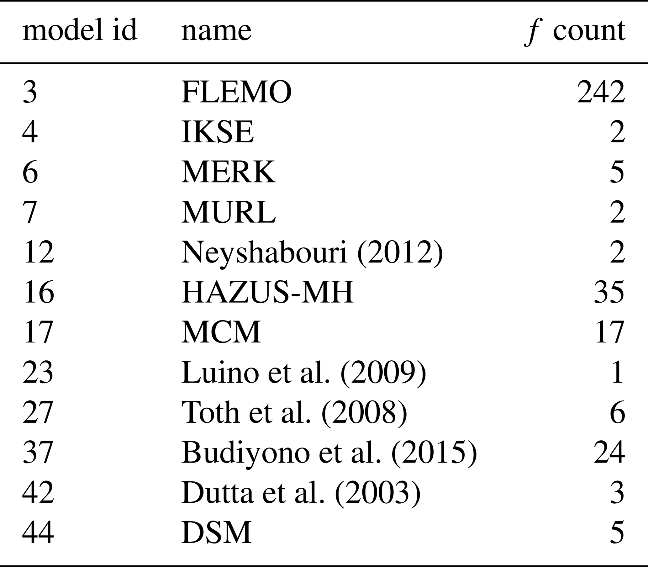
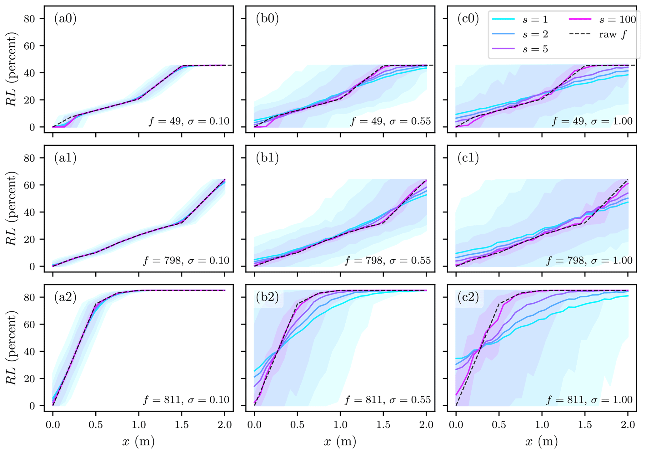
Figure 1 Relative loss vs. anchor depth (x_b) for three example functions and three synthetic depth generation standard deviations (σ) computed against the depth values and aggregation (s) described in the text. Shaded areas show the corresponding q₉₅ and q₅ for the RL computed for each level of aggregation. Functions are from model 3, 3 and 37 from Table 1 for panel (a), (b), and (c) respectively.

2.2 Synthetic Depths Generation

Each of the 344 selected discrete functions have a distinct shape, depth domain (from −1.22 to 10 m), and relative loss domain (from 0.0 to 116, with a value greater than 100 indicating damages more severe than the estimated replacement value). In practice, each asset (e.g., house) would have its flood damage calculated with a specific function and the exposure variables (e.g., depth) sampled for each flood event. Under aggregation, multiple assets would be collapsed to a single node prior to function computation. The exposure (and vulnerability) indicators of this collapsed asset are generally computed through averaging of the original, singular assets. To provide a comprehensive analysis of the full range of exposure depths supported by each function, a range of depth values are generated using a normal distribution and then sampled and averaged according to the level of aggregation.

To generate the synthetic depth values, the independent variable domain (depths) is discretized from 0.0 to 2.0 to produce 30 anchor depth values (x_b). Each of these x_b values is used as the average or mean depth under evaluation, with lower values representing shallower floods and higher values (closer to 2.0) very deep floods. To represent the variance in depths within a group of assets for a given flood, raw synthetic depth values are then randomly generated around each x_b by sampling 2000 points from three normal distributions ($N[\mathit{\sigma }=(\mathrm{0.1},\mathrm{0.55},\mathrm{1.0}),\mathit{\mu }=x_b]$). Higher variances (σ²) represent steeper terrain and water surface gradients, while lower values represent flatter areas like a lowland floodplain. These raw values are then aggregated by randomly splitting the 2000 depth values into N₁₂ groups of size $s_j=(\mathrm{1},\mathrm{2},\mathrm{5},\mathrm{100})$ and computing the mean. In this way, 360 arrays of synthetic depth values covering a broad range of flood magnitudes, variance, and levels of aggregation are prepared.

Figure 2 Relative loss error for three levels of aggregation (s) and three synthetic depth families (σ) for a selection of the models described in Table 1. Faint circles show each function (f) while the bold circles show the function ensemble mean for that model.

2.3 Relative Loss Errors

Using each of the 360 synthetic depth arrays on each of the 344 functions, a set of relative loss arrays (RL${}_{x_b,s_j,\mathit{\sigma },f}$) is computed, each associated with an anchor depth value (x_b), a level of aggregation (s), a standard deviation (σ) and a flood damage function (f). To compute the aggregation error potential of each function under various flood conditions, arrays are grouped by function (f), standard deviation (σ), and aggregation level (s). For each of these groups, the mean of the relative loss values is plotted against x_b. Second, for each of these four series, the area against the un-aggregated result is calculated as:

$$\begin{array}{}\text{(2)}& e_{s_j,\mathit{\sigma },f}=\underset{x=\mathrm{0}}{\int }\stackrel{\mathrm{‾}}{\mathrm{RL}\left[x,s_{\mathrm{1}},\mathit{\sigma },f\right]}-\stackrel{\mathrm{‾}}{\mathrm{RL}\left[x,s_j,\mathit{\sigma },f\right]}\end{array}$$

where e is the aggregation error potential and the integrals are evaluated using the composite trapezoidal rule, a common method for estimating the area under a curve by discretizing into trapezoids (NumPy Developers, 2022).

Figure 3 Aggregation error potentials calculated with Eq. (2) for each function (f) of the models described in Table 1.

3 Results and Discussion

Three example damage functions (f) are shown in Fig. 1 along with the mean and two quantiles (q₉₅ and q₅) of the resulting loss values computed under four levels of aggregation against the generated depth values. These three damage functions were selected to demonstrate typical behaviour present in all functions. Looking from left-to-right, Fig. 1 shows how large variances (σ²) employed in the synthetic depth generation act to spread the resulting relative loss values. Working in a similar but opposite manner, large aggregations (s) reduce the spread of relative loss values. This is intuitive if we consider that the averaging employed in the aggregation works like a filter to reduce variance.

A clock-wise rotation can also be seen in Fig. 1, where series with less aggregation (e.g., s=0) have positive/negative deviation from the left/right tails of the raw functions. This can be explained by the treatment of out-of-range depth values (x). As explained above, when a synthetic depth value with negative exceedance is calculated (i.e., less than the minimum (x) provided in the lookup table), a relative loss of zero is returned. Away from these x range limits (e.g., x_b=1.0), the normally distributed synthetic depths yield roughly similar positive and negative residuals from the monotonically increasing functions, which balance during the averaging. On the other hand, closer to the x range limits (e.g., x_b=0.0) the residuals become unbalanced as those x values exceeding the range (e.g., x_b<0.0) lose their relation with RL while those within range maintain the relation. At the low end of the range (e.g., x_b=0), this phenomena produces a bias negatively related to aggregation and positively related at the high end (e.g., x_b=2.0). This is intuitive if we consider the aggregated synthetic x values (i.e., s>1) have had their variance reduced (through averaging), meaning fewer extreme x values and therefore the RL imbalance discussed above is less severe with aggregation. Because the depth values considered here are generated with a normal distribution, it is likely that some x values for low anchor depths (e.g., x_b=0.0) would be below ground in a real flood risk model (some negative x values are realistic as buildings are typically elevated slightly above ground). In cases where such ground water exposure is ignored or negligible (the case of most models), the bias around low anchor depths would be smaller than what we report here. A similar, but weaker argument could be made for large x_b values which traces back to the suitability of a normal distribution for representing exposure depths. This important issue was not investigated as part of our first order approximation.

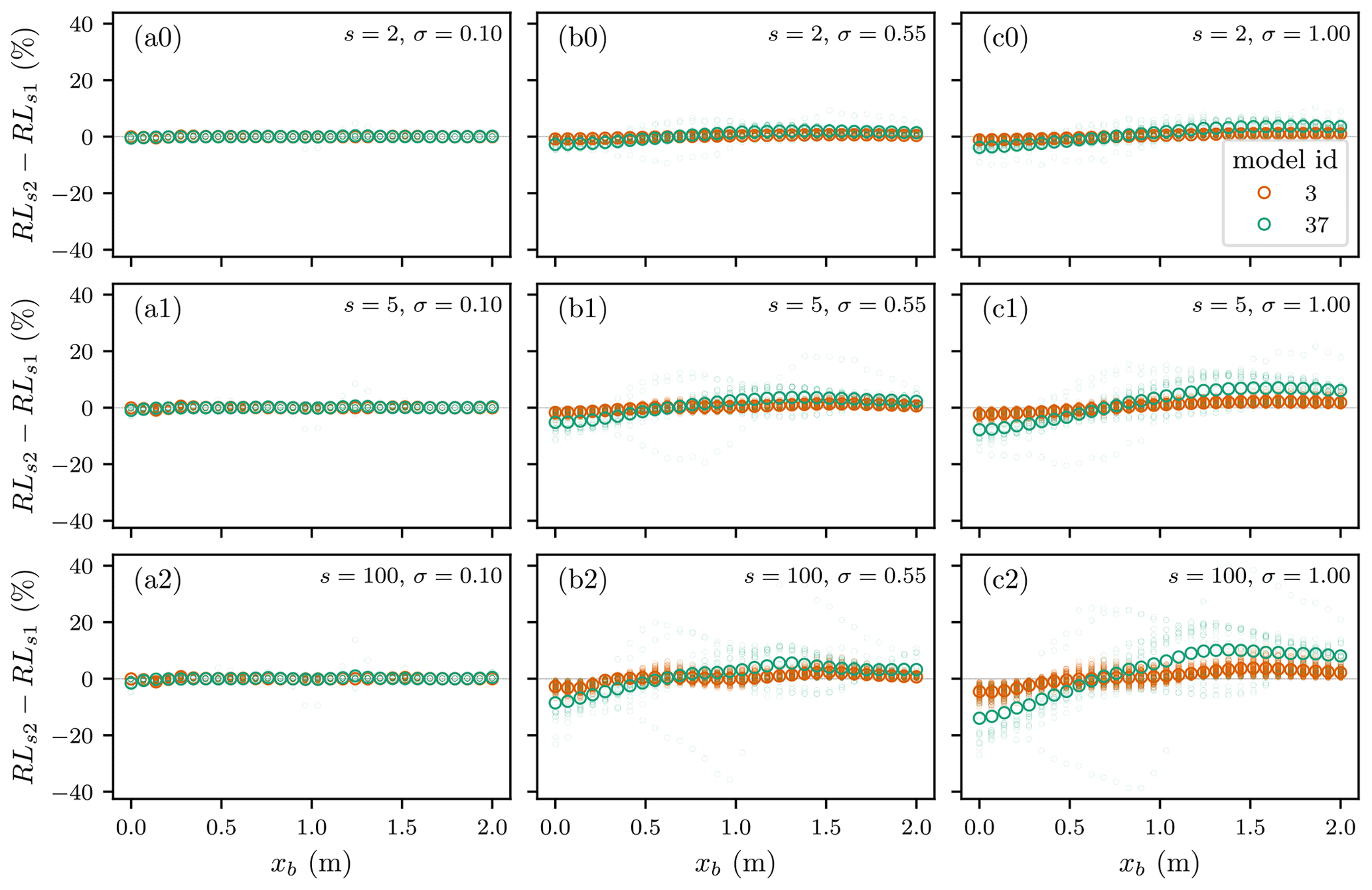
Figure 2 shows the error in relative loss as a function of x_b for two example models from Table 1, each containing a set of damage functions. These models were selected to demonstrate behaviour present in all models. This shows that the sensitivity to aggregation errors varies by model or damage function (f). This is intuitive considering the diverse function shapes reported by Gerl et al. (2016). Looking at the general increase in absolute error magnitude from top left to bottom right of Fig. 2 suggests a positive relation with variance in depth values (σ²) and the level of aggregation (s). This aligns with our understanding of Jensen's inequality if we consider that larger variances (σ²) and aggregation both lead to a more severe compression of tail values about the mean. Figure 2 also shows that errors can be significant, approaching 40 % relative loss for the most extreme case considered here. In contrast, when variance in depth values (σ²) is low, as in flat floodplains, the majority of functions have relative loss errors less than 5 % for the most extreme level of aggregation considered here (s=100).

Examining the relation of error to x_b, Fig. 2 suggests generally negative errors for small depths (x_b<1.0) and positive errors for larger depths (x_b>1.0). This can be explained by the treatment of out-of-range depth values (x) and the clock-wise rotation shown in Fig. 1. The implications of this depth-dependent error could be significant for flood risk analysis aimed at informing flood protection investment decisions where a broad range of flood event magnitudes are assumed to have roughly similar errors (IWR and USACE, 2017). However, the significance of these findings is limited by our first order approach for generating synthetic depths from a normal distribution, which may not represent real exposure depths well.

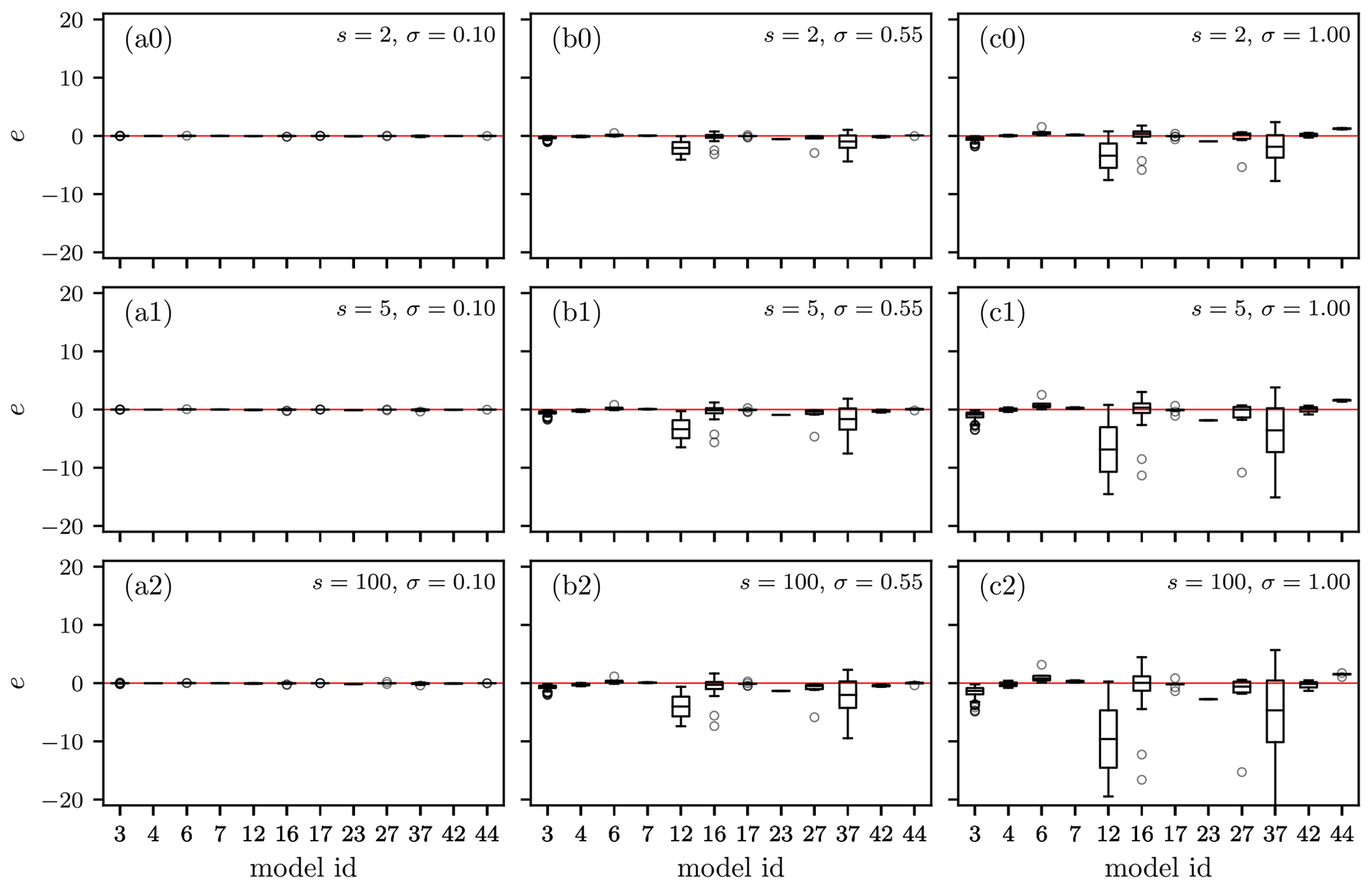
To provide a simple metric for the 344 functions covered in Table 1, Eq. (2) was used to compute the total area of each error series (similar to what is shown in Eq. 2). The resulting aggregation error potentials are shown in Fig. 3. This shows that the sensitivity to aggregation errors varies widely between models and even between damage functions (f) within the same model. This is intuitive considering the diverse function shapes and the harmonization of variables necessary to directly compare the different models. Further, Fig. 3 shows the majority of models have mean error (e) values below zero, suggesting an overall negative bias across the full depth domain.

4 Conclusions

To better understand the potential and magnitude of errors introduced through averaging of flood risk models, a novel first order evaluation of 344 flood damage functions was performed using synthetically generated depth data. While the character and magnitude of aggregation errors will depend on the specifics of a given flood risk model, the general approach applied here demonstrates that low-depth floods tend to have negative errors while high-depth floods have positive errors. Further, we demonstrate that overall, error tends to be negative for the 344 damage functions considered.

The findings reported here provide useful information for flood risk modellers evaluating the appropriateness and extent of aggregation to include in their models. For example, in areas with high depth variance where models with large aggregation error potential (e on Fig. 3) are to be applied, aggregation should be minimized. While this can be difficult, minimizing aggregation can be achieved by constructing damage models where assets (e.g., buildings) are treated as individual elements within the model (rather than aggregated elements). Finally, this work demonstrates the potential severity of aggregation errors and how poorly these are understood, and therefore the need for further study.

Future work should evaluate the performance of the normal distribution applied here to synthetically generate depths. Also, a more generalizeable measure of curvature (e.g., local derivative) could be explored to more clearly classify and communicate the aggregation error potential of different functions. By extending the first order approximations developed here, the flood risk model domain could be segregated into areas with more or less sensitivity to aggregation errors. In this way, the accuracy of large-scale flood risk models could be improved without drastically increasing the computational requirements.