Seasonal precipitation forecasting with large scale climate predictors: a hybrid ensemble empirical mode decomposition-NARX scheme

Much of northern Tunisia regularly experiences extremes of drought and flooding, with high rainfall variability. The development of reliable and accurate seasonal rainfall forecasts can provide valuable information to help mitigate some of the outcome of floods and enhance water management and monitoring, particularly for agriculture. Whether climate indices oscillations contain some information to be useful for hydrological forecasting is worth investigating. Ensemble monthly rainfall forecasts are carried out using a hybrid neural network model. The hybrid model called EEMD-NARX based on a non-linear autoregressive network with exogenous inputs (NARX) coupled to Ensemble Empirical Mode Decomposition (EEMD) method is developed in this work. First, the EEMD is performed to extract significant information from modes of variability (IMF) associated to climate indices and precipitation. Each IMF of selected indices as well as precipitation IMFs are then used as inputs to the NARX forecasting model to forecast each IMF of precipitation. To make forecasts operational, we reconstruct precipitation by summing of all forecasted IMFs to make comparison with observed precipitation in the Medjerda river basin located in north Tunisia. Results show that IMFs of MEI and SOI indices can be distinguished from a white noise at the 95 % level. It is also found that an oscillatory forcing coming from the Atlantic influences the precipitation in the Mediterranean basin. The results indicate that exogenous inputs like climatic indices improve the accuracy of forecasts in some in some precipitation stations. The correlation coefficient between observed and forecasted monthly precipitation is ranging from 0.7 to 0.8. EEMD allows extracting significant components from exogenous inputs like climate indices that help reducing predictive uncertainty as well as improving forecasts of a NARX model at longer lead-times.

1 Introduction

Precipitation forecasting is useful for water resources and hydraulic structures management. Extreme events have devastating consequences that disfigure the nature and cause thousands of casualties. For new monitoring, good management and forecasting of floods, it is essential to go through a precipitation forecasting. Seasonal forecasting is useful for the agricultural sector which is among the key sectors of the Tunisian economy. The precipitation process is difficult to understand and to model because of the complexity of the phenomena and the atmospheric processes that generate it. Then a reliable forecast of the precipitation remains a challenge. Several methods could be used for precipitation forecasting from statistical to empirical models through the artificial intelligence models. Artificial neural networks (ANN) are robust tools for modeling and forecasting many of the nonlinear hydrological processes but their performance remains linked to the complexity of the network. Improving the performance of a neural network model can be obtained with a preprocessing of the input and output data. Among the signal preprocessing methods we found the Empirical Mode Decomposition (EMD) (Huang et al., 1998). It is one of the methods in the frequency domain that can process non-linear and non-stationary data. An application of this approach applied to environmental data analysis: rainfall, temperature, wind and streamflow analysis is presented in Rao and Hsu (2008). Kisi et al. (2014) reported the use of ANNs in forecasting hydrological variables as well as combined methods with ANNs. In their work, the EMD-ANN model was compared with the single ANN model. The optimal test results were obtained for the three-input to EMD-ANN model. Liang et al. (2021) proposed three hybrid models that couple varied pre-processing methods, which are empirical mode decomposition (EMD), ensemble empirical mode decomposition (EEMD), and empirical wavelet transform (EWT), with the nonlinear autoregressive networks with exogenous inputs (NARX) were applied to forecast tidal level.

In spite of the generalization ability of ANNs and due to the nonlinear and non-stationary nature of the rainfall time series, it is necessary the search for analysis alternatives that improve the accuracy of predictions. Basha et al. (2015) developed a stochastic model that reproduces non-stationary oscillation (NSO) processes by employing ensemble empirical mode decomposition (EEMD) and non-parametric techniques to predict the evolution of temperature, precipitation and soil moisture. Ouachani et al. (2013) studied the effect of climate variability on precipitation in the Medjerda basin and found that indices related to ENSO as well as Mediterranean Oscillation have potential power in forecasting.

Could exogenous inputs such as climate indices, defined as difference between sea surface temperature or sea level pressure between two different localizations in the sea, add some additional information to an ANN based EEMD model is the question that we will try to respond.

The remaining part of the paper is organized as follows. The proposed methodology is detailed in Sect. 2, where a brief description of Empirical Mode Decomposition (EMD), EEMD, backpropagation scheme and NARX are also presented. Section 3 presents the hydro-climatic data and Sect. 4 the obtained results. Finally, the paper is concluded in Sect. 5.

2 Methodology

This paper proposes a hybrid model for long term rainfall forecasting, adopting the Ensemble Empirical Mode Decomposition (EEMD), and as a forecasting tool, the Nonlinear AutoRegressive with eXogenous (NARX) input network. The two methods are described below.

2.1 The Ensemble Empirical Mode Decomposition (EEMD) method

As discussed in Blöschl et al. (2019), in UPH18, we need to extract information from available data in order to inform the building process of hydrological forecasting models. EMD is a nonparametric method that aims to decompose a signal into a set of meaningful components called intrinsic mode functions (IMFs). The complete mathematical description of the empirical mode decomposition is beyond the scope of this article, but can be found in Huang et al. (1998). A brief description of the algorithm can be made. The EMD extracts a series of IMFs that must respect two criteria: (1) for each IMF, the number of local extrema and the number of zero-crossings are equal or differ at most by one; (2) at any time and for every IMF, the mean value of the envelope defined by the local minima and the local maxima is zero. The criterion (1) forces an IMF to evolve as a series of periodic fluctuations and prevents the superposition of multiple oscillations. The criterion (2) imposes a null trend to the IMFs and is necessary to obtain IMFs with periodic zero-crossings as imposed by the criterion (1). The process to extract an IMF is called sifting. The sifting process gives the following final decomposition:

$$\begin{array}{}\text{(1)}& X={\sum }_{j=\mathrm{1}}^q{C}_j+r.\end{array}$$

Where C_j with $j=\mathrm{1},\mathrm{2},\mathrm{\dots },q$ are the IMFs and r is the residue trend.

To verify whether IMFs contain exact signal or simply noise, Wu and Huang (2004) established a statistical significance test (at any given statistical confidence level) based on the relationship between the energy and the mean period of each component. Wu and Huang (2009) proposed the ensemble method by sifting an ensemble of white noise-added signal and treats the mean as the final true result. The EEMD requires two parameters: the variance of the added noise and the number of samples. To calculate the average of each IMF, their total number must be known. The approximate dyadic properties of EMD suggest that the total number of IMFs should be close to log 2(N), where N is the number of observations (Wu and Huang, 2009). The stopping criterion is generally a fixed number of iterations (e.g. 10).

2.2 Artificial Neural Network

The ANNs have been widely used in the scientific field of time series prediction due to their inherent nonlinearity and high robustness in noise. Typically, the challenge task of time series prediction can be expressed as finding the appropriate function F so as to acquire an estimate $\widehat{y}(t+D)$ of the time series y at time t+D ($D=\mathrm{1},\mathrm{2}\mathrm{\dots }$) given the past values of y up to time t, plus the values of exogenous input x:

$$\begin{array}{}\text{(2)}& \widehat{y}(t+D)=F\left(y\left(t\right),\mathrm{\dots },y(t-d_y),x\left(t\right),\mathrm{\dots },x(t-d_x)\right)\end{array}$$

where y(t) and x(t) represent the values of y and x in time t respectively. The variables d_y and d_x are the lag time parameters of model and in case of D=1 we have the one step ahead prediction of time series y.

In this paper, we apply the backpropagation NN learning algorithm, which includes four main steps as: feed forward computation, backpropagation to the output layer, backpropagation to the hidden layer and weight updates. This forecasting engine has good abilities for dealing with nonlinear systems, such as forecasting problem of precipitation. The structure of the NN is a three layered back propagation NN with one input layer, one hidden layer and one output layer.

For each hidden neuron j (in the hidden layer), the input xj and output yj are defined as:

$$\begin{array}{}\text{(3)}& {\displaystyle }{\widehat{x}}_i=\sum _{i=\mathrm{1}}^n{w}_{ij}{y}_i\text{(4)}& {\displaystyle }{\widehat{y}}_j=F\left({\widehat{x}}_j+h_j\right)\end{array}$$

where w_ij is the weight between the ith neuron in the input layer and j^thneuron in the hidden layer; F(.) is the activation function of the hidden neurons; ${\widehat{x}}_i$ and ${\widehat{y}}_j$ are the output of input neuron i and hidden neuron j; h_j is the bias of hidden neuron j. The initial number of neurons in the hidden layer is considered. In this work, the learning rule used to adjust the NAR weights is based on the Levenberg-Marquardt method, one of the BP algorithms. It is being more powerful and faster than the conventional gradient descent techniques.

2.3 Proposed EEMD-NARX model

The overall procedure for EMD-NARX is given below:

• 1.

  Decompose the concerned time series (X_t) into a finite number of intrinsic mode functions (IMFs).

• 2.

  Select significant IMF components using significance test.

• 3.

  Calibrate the NARX model using each IMF_i of the selected indices and precipitation as inputs to predict IMF_iof the precipitation. Validate the model using data from the validation period.

• 4.

  Predict the IMF components using the calibrated and validated NARX model with the best performance in the validation period.

• 5.

  Sum up the forecasted IMFs from each model.

The model is run 100 times using the bootstrap procedure that adds noise with known standard deviation equal to 0.2 to the output. The mean of the obtained ensembles represent the forecasting value. For all the 100 experiments, the performance measure of the mean is computed and thus a reliable estimate of the performance is obtained. For NARX, three layers are considered: one input layer, one hidden layer and one output layer. Several network architectures are tested by varying the number of nodes in the hidden layer from 5 to 20. The architecture with the best performance in the validation period is used to make forecasts.

Among the model efficiency criteria in the literature, the coefficient of determination (R²) and the Nash–Sutcliffe coefficient (NASH) (Eq. 5) of efficiency are the most commonly employed performance evaluation criteria and are also found to be good evaluation criteria by experts.

$$\begin{array}{}\text{(5)}& \text{NASH}=\mathrm{1}-{\displaystyle \frac{\sum _{i=\mathrm{1}}^n(y_i-{\widehat{y}}_i{)}^{\mathrm{2}}}{\sum _{i=\mathrm{1}}^n(y_i-\stackrel{\mathrm{‾}}{y}{)}^{\mathrm{2}}}}\end{array}$$

where n refers to the total number of observations; ${\widehat{y}}_i$, y_i, $\stackrel{\mathrm{‾}}{y}$ represent the predicted monthly precipitation, observed precipitation, and the mean observed precipitation data, respectively.

The Willmott index of agreement (IOA) (Eq. 6) is also used

$$\begin{array}{}\text{(6)}& \text{IAO}=\mathrm{1}-{\displaystyle \frac{\sum _{i=\mathrm{1}}^n({\widehat{y}}_i-y_i{)}^{\mathrm{2}}}{\sum _{i=\mathrm{1}}^n{\left(\left|{\widehat{y}}_i-\stackrel{\mathrm{‾}}{y}\right|+\left|y_i-\stackrel{\mathrm{‾}}{y}\right|\right)}^{\mathrm{2}}}}\end{array}$$

IOA equal to 1 is being perfect score. It is sensitive to the difference between the mean of ${\widehat{y}}_i$ and y_i as well as the difference between the standard deviation of ${\widehat{y}}_i$, y_i.

3 Hydro-climatic data

The analysis of the monthly precipitation is carried out for six rainfall stations reported in Ouachani et al. (2013) associated with the upper part of the Medjerda river basin (Fig. 1), a trans-boundary river, located in northern Tunisia and which accounts for the Mediterranean water budget in the Blue Plan (Margat and Treyer, 2004). The water resources and agricultural potential of this region is crucial for the Tunisian economy. Therefore, the new monitoring, modelling and optimal management of these resources is of primary importance. Field observation of rainfall is provided by the National Water Resources Division of Tunisia. These rainfall stations were chosen for their long-term records (generally exceeding 50 years) and for their good data quality. Four climate indices; the Multivariate Enso Index (MEI), Southern Oscillation Index (SOI), North Atlantic Oscillation (NAO) and Mediterranean Oscillation Index (MOAC) are used in this work as suggested by Ouachani et al. (2013). The common period 1950 to 2011 between series is chosen. Before analysis, the precipitation and climate indices time series are standardized, by subtracting the mean and dividing by the standard deviation, to ensure a comparable scale.

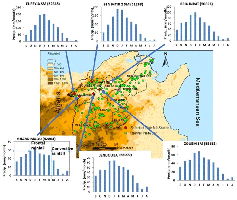
Figure 1 Geographic map of selected Rainfall stations in the Medjerda river basin with each seasonal precipitation.

4 Results

4.1 Decomposition of precipitation using EEMD

The data is decomposed into IMFs by using the Matab code of EEMD method provided by Wu and Huang (2009) with 100 ensembles and a noise level of 0.2. The monthly precipitation data recorded at Ghardimaou (52864) for the period 1950–2011 is shown in Fig. 2 as well as a total of 8 components and the residue. The first component (C1) which has a very high frequency is generally considered as noise. The last component (C8) represents the trend. C4 to C6 show a long-term oscillation with asymmetrical changes. While C7 represents the 40-year oscillation. The IMFs are subjected to the significance test and are plotted in Fig. 3a. The result of the significance test indicates that the three IMFs C2, C3 and C5 can be considered as real oscillatory components and are distinguishable from random noise. However, the other components are not statistically significant. The test of significance is performed also for climate indices. I can be shown for example from Fig. 3b and c that all IMFs related to MEI can be distinguished from a white noise at the 95 % level while only the second component IMF2 of SOI is not significant. All these components can be used as inputs to the forecasting model. Here we can focus on the UPH17 (Blöschl et al., 2019) and how data preprocessing methods can help extract significant components from traditional hydrological observations. NAO and MOAC components on medium time scales (IMF3, IMF5) are well correlated to precipitation components with 6 months delay time. It can be concluded that the negative phase of NAO as a tendency to generate precipitations in the winter season. As discussed in the previous section, the significant components as well as the other components are forecasted by a NARX model.

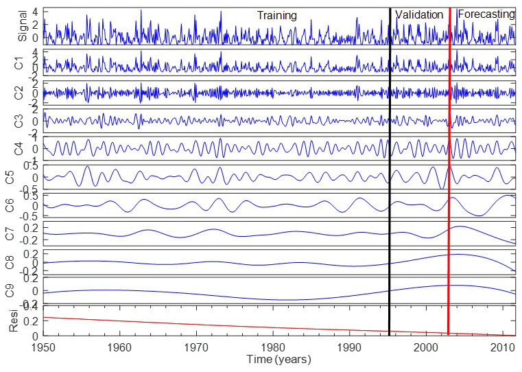
Figure 2 Monthly precipitation anomaly data recorded from 1950 to 2011 at station Ghardimaou (52864) in the Medjerda basin decomposed into IMFs (blue lines) and a residue (red line) using EEMD. Where the calibration period from 1950 to 1995. The period 1995–2003 is for the validation and the period 2003–2011 is used to validation.

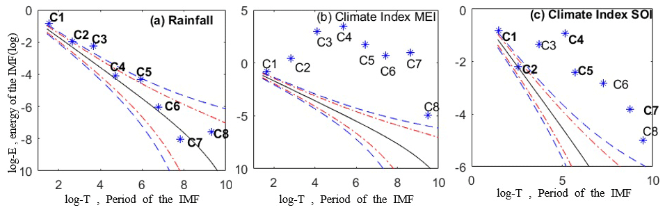
Figure 3 Significance test of the extracted IMFs for (a) precipitation station Ghardimaou (52864), (b) climate index MEI and (c) climate index SOI with 95 % (red line) and 99 % (blue line) confidence limits. Each point (*) below the lines indicates that the hypothesis that the corresponding IMF of the observed series is not distinguishable from the corresponding IMF of a random noise series cannot be rejected with the confidence levels (95 % and 99 % respectively).

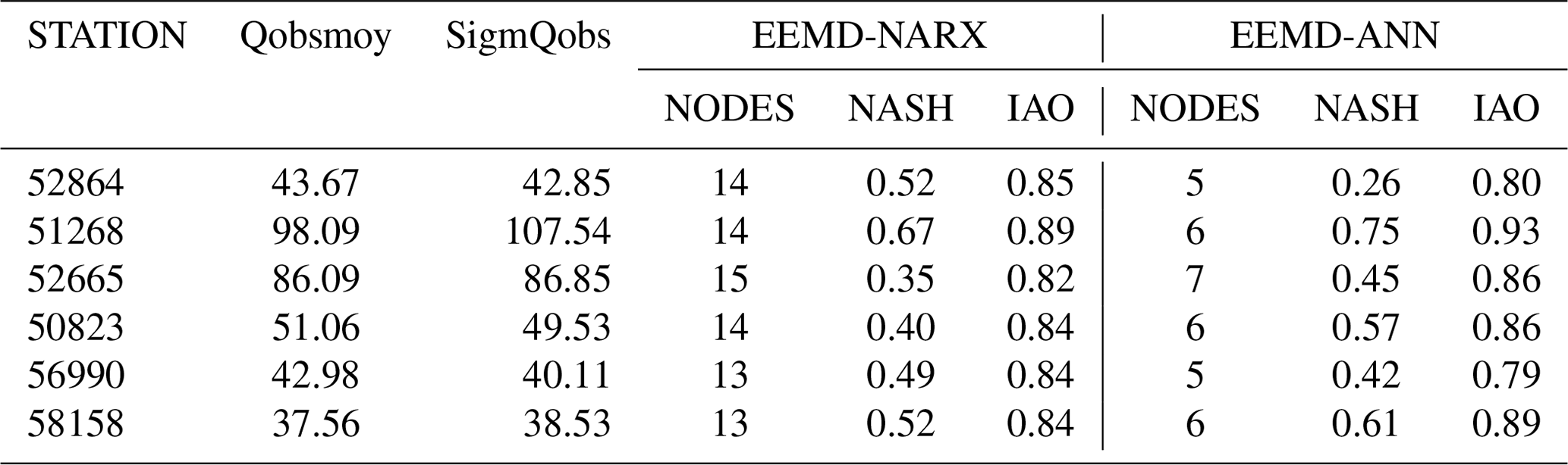
Table 1 Performance evaluation of the precipitation forecasts by the EEMD-NARX and EEMD-ANN models.

4.2 Forecasting model based EEMD

The data are divided by block into three parts for training, validation and test (forecast), respectively assigning 60 %, 20 %, 20 %. Two models are compared. The first one (EEMD-NARX) uses a set of inputs constructed from climate indices and precipitation with time delay ranging from 1 to 12 months. The second model (EEMD-ANN) has only precipitation as inputs. Table 1 summarizes the performance criteria estimates for the (EEMD-NARX), which is compared against an EEMD-ANN model for the original signal without exogenous inputs. From this we can observe good forecasts. All performance indices are in accordance. It can be observed good IAO coefficients exceeding 0.8. When the EEMD-ANN scheme is unable to give good forecasts, the EEMD-NARX outperforms a considerable difference. This is shown in the case of station Jendouba (56990) and Ghardimaou (52864) in gray color row. The IAO criteria grow from 0.80 to 0.85.

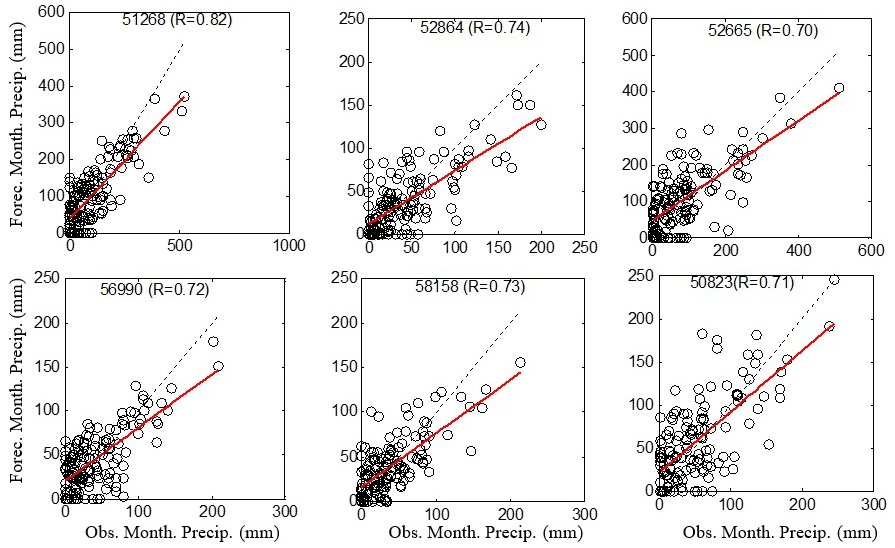
Figure 4 Regressions of forecasted precipitation using EEMD-NARX model versus observed precipitations (circles) in the period 2003 to 2011 with the correlation coefficient for each station used in the study. The red line is the linear regression while the black dot line is the first bisector.

Regressions of forecasted precipitations using (EEMD-NARX) versus observed data precipitation shown in Fig. 4 reveal good forecasts of the monthly precipitation with correlation exceeding 0.7 for all stations. Results are comparable to those found by Kisi et al. (2014). However we notice the disability of the model to forecast the highest values of precipitation as the regression line is under the y=x line. In addition the model overestimate low values as zero crossing value of the regression line is positive in all stations. All IFMs are well forecasted except IMF1 who can be distinguished from the others. The first IMF is the decomposition of the signal in the very high frequency and contains some noise even if it explains the precipitation signal as shown by the significance test. As reported by Kisi et al. (2014), because, the IMF1 component is characterized by higher mean frequencies and include noise component because EMD acts a filter bank for Gaussian noise, white noise and turbulence of time series. Therefore, forecasting of IMF1 component is difficult.

5 Conclusions

To forecast the future tendencies of nonlinear and nonstationary precipitation time series, a hybrid intelligent forecasting model is proposed, which is based on EEMD and ANN. EEMD allows extracting significant components to help reducing predictive uncertainty as well as improving forecasts of a neural network model. According to the obtained results, the EEMD-NARX scheme improves the forecasting results and offers a simple approach for the stable prediction of non-stationary data when an EEMD-ANN is unable to give good forecasts. It can be concluded that exogenous inputs like climate indices can add some additional information to enhance monthly precipitation forecasts. As a future work, it would be interesting to explore the possibility of employing different aggregation methods. Because the forecast of IMF1 is difficult, it would be useful to perform a comparison with wavelet decomposition. The hybrid model has a good generalization performance and long-term forecasting ability.