Pros and cons of various efficiency criteria for hydrological model performance evaluation

Confidence in hydrological predictions is linked to the model's performance in reproducing available observations. However, judgment of a model's quality is challenged by the differences which exist among the available efficiency criteria or objective functions. In this study, model outputs based on several objective functions were compared and found to differ with respect to various circumstances of variability, number of outliers, and model bias. Computational difficulty or speed of a model during calibration was shown to depend on the choice of the efficiency criterion. One source of uncertainty in hydrological modelling is the selection of a particular calibration method. However, this study showed that the choice of an objective function is another sub-source of calibration-related uncertainty. Thus, tackling the issue of uncertainties on model results should comprise combination of modelled series obtained based on (i) various objective functions separately applied to calibrate a model, (ii) different calibration methods, and (iii) several hydrological models. The pros and cons of many new and old efficiency criteria which can be found explored in this study highlight the need for modellers to understand the impact of various calibration-related sub-sources of uncertainties on model outputs.

1 Introduction

Model quality can be judged in terms of “goodness-of-fit” (GOF) or how well a model fits through observations or measured data points (Onyutha, 2022). Mathematical measures of model quality can be regarded as efficiency criteria (Beven, 2012). There are several efficiency criteria such as coefficient of determination (R²) (also called R-squared), revised R-squared (RRS) (Onyutha, 2022), index of agreement (IOA) (Willmot, 1981), Nash Sutcliffe efficiency (NSE) (Nash and Sutcliffe, 1970), Kling Gupta efficiency (KGE) (Gupta et al., 2009), hydrological model skill score or Onyutha Efficiency (OE) (Onyutha, 2022), Liu mean efficiency (LME) (Liu, 2020), Taylor skill score (TSS) (Taylor, 2001), Root mean squared error (RMSE), and Mean absolute error (MAE). Differences exist among these various efficiency criteria and/or objective functions. Furthermore, each efficiency criterion has its advantages and disadvantages. Thus, outputs of a model calibrated using various objective functions can also differ.

Question number 20 of the unsolved problems in hydrology (UPH 20) (Blöschl et al., 2019) deals with the need to reduce model uncertainty. As highlighted in UPH20, uncertainty in model results can be due to model structure, parameter, or inputs. However, other sources of model uncertainty also exist as explored in this study.

It is worth noting that many old and new efficiency criteria can be found in literature. However, no any paper (which explored the pros and cons of the various old and new efficiency criteria) could be found in literature by the time of conducting this study. Therefore, this study was aimed at filling this knowledge gap to give modellers wide-ranging information which could influence decision regarding the choice of the best performing model in making hydrological prediction.

2 Materials and methods

2.1 Data and models

To evaluate efficiency criteria, several series were required. One way to obtain the required series for analysis was to make use of outputs from hydrological models. Here, conceptual models were preferred to physical models. This was because conceptual models (i) have few parameters, (ii) require few inputs, and (iii) are easy to calibrate compared with physical models. In this line, two lumped conceptual hydrological models including Hydrological Model focusing on Sub-flows' Variation (HMSV) (Onyutha, 2019) and Nedbør-Afstrømnings-Model (NAM) (Nielsen and Hansen, 1973) were applied to model river flow of the Jardine River catchment (with area 2500 km²) in Australia. Each of the selected models require catchment-wide averaged rainfall and potential evapotranspiration as inputs.

2.2 Application of the selected hydrological models

Each selected model was calibrated using the Generalized Likelihood Uncertainty Estimation (Beven and Binley, 1992) framework. To do so, one of the metrics (R², RRS, IOA, NSE, KGE, OE, LME, TSS, RMSE, and MAE) was selected as the objective function for model optimization by running HMSV or NAM using 10 000 sets of parameters randomized within the stipulated parameter space. The optimal set of parameters was that which yielded the best value of the objective function or the most promising fit between the observed and modelled series. The procedure was repeated to ensure each of the efficiency criteria was used to generate a set of model outputs. Finally, model outputs based on the various efficiency criteria were compared.

To compute the various efficiency criteria, consider $\overline{X}$ and $\overline{Y}$ as the mean of the observed (X) and modelled (Y) series, respectively. Take r as the coefficient of correlation between X and Y. Let r_a denote the maximum attainable r value (and it was taken to be 0.9975 in this study). Other terms to note include sample size (n), standard deviation of X (s_x), variance of $X\left(s_x^{\mathrm{2}}\right)$, standard deviation of Y(s_y), variance of $Y\left(s_y^{\mathrm{2}}\right)$, normalized $s_y\left({\widehat{s}}_y\right)$, distance covariance of X (d_xx), distance covariance of Y (d_yy), and distance covariance of X and Y (d_xy). We can compute the selected efficiency criteria using

$$\begin{array}{}\text{(1)}& {\displaystyle }{R}^{\mathrm{2}}=\sum \left(X-\overline{X}\right)\left(Y-\overline{Y}\right)/\sqrt{\sum {\left(X-\overline{X}\right)}^{\mathrm{2}}\sum {\left(Y-\overline{Y}\right)}^{\mathrm{2}}}\text{(2)}& {\displaystyle }\mathrm{RRS}=\mathrm{|}r\mathrm{|}\times {\displaystyle \frac{\min (s_x,s_y)}{\max (s_x,s_y)}}\times {\displaystyle \frac{\min (s_x^{\mathrm{2}},s_{yc}^{\mathrm{2}})}{\max (s_x^{\mathrm{2}},s_{yc}^{\mathrm{2}})}}\end{array}$$

where $s_{yc}^{\mathrm{2}}=(n-\mathrm{1}{)}^{-\mathrm{1}}\times \sum {\left(Y-\overline{X}\right)}^{\mathrm{2}}$

$$\begin{array}{}\text{(3)}& {\displaystyle }\mathrm{IOA}=\mathrm{1}-{\displaystyle \frac{\sum {\left(X-Y\right)}^{\mathrm{2}}}{\sum \left(\mathrm{|}(X-\overline{X}\right)\mathrm{|}+\mathrm{|}\left(Y-\overline{Y}\right)\mathrm{|}{)}^{\mathrm{2}}}}\text{(4)}& {\displaystyle }\mathrm{NSE}=\mathrm{1}-{\displaystyle \frac{\sum {\left(X-Y\right)}^{\mathrm{2}}}{\sum {\left(X-\overline{X}\right)}^{\mathrm{2}}}}\text{(5)}& {\displaystyle }\mathrm{KGE}=\mathrm{1}-\sqrt{{\left(r-\mathrm{1}\right)}^{\mathrm{2}}+{\left({\displaystyle \frac{s_y}{s_x}}-\mathrm{1}\right)}^{\mathrm{2}}+{\left({\displaystyle \frac{\overline{Y}}{\overline{X}}}-\mathrm{1}\right)}^{\mathrm{2}}}\text{(6)}& {\displaystyle }\mathrm{OE}=r_d\times {\displaystyle \frac{\min (d_{xx},d_{yy})}{\max (d_{xx},d_{yy})}}\times {\displaystyle \frac{\min (s_x^{\mathrm{2}},s_{yc}^{\mathrm{2}})}{\max (s_x^{\mathrm{2}},s_{yc}^{\mathrm{2}})}}\end{array}$$

such that $r_d=d_{xy}\times {\left(\sqrt{d_{xx}\times d_{yy}}\right)}^{-\mathrm{1}}$

$$\begin{array}{}\text{(7)}& {\displaystyle }\mathrm{LME}=\mathrm{1}-\sqrt{{\left({\displaystyle \frac{s_y}{s_x}}\times r-\mathrm{1}\right)}^{\mathrm{2}}+{\left({\displaystyle \frac{\overline{Y}}{\overline{X}}}-\mathrm{1}\right)}^{\mathrm{2}}}\text{(8)}& {\displaystyle }\mathrm{TSS}={\displaystyle \frac{\mathrm{4}(\mathrm{1}+Q_d)}{{\left({\widehat{s}}_x+\frac{\mathrm{1}}{{\widehat{s}}_y}\right)}^{\mathrm{2}}(\mathrm{1}+r_{\mathrm{a}})}}\end{array}$$

while $Q_d=\sum \left(X-\overline{X}\right)\left(Y-\overline{Y}\right)/\left(n\times s_x{s}_y\right)$

$$\begin{array}{}\text{(9)}& {\displaystyle }\mathrm{RMSE}=\sqrt{n^{-\mathrm{1}}\times \sum {\left(X-Y\right)}^{\mathrm{2}}}\text{(10)}& {\displaystyle }\mathrm{MAE}=n^{-\mathrm{1}}\times \sum \left(\mathrm{|}X-Y\mathrm{|}\right)\end{array}$$

Note that in Eqs. (2) and (6), when $s_x=s_{yc}=\mathrm{0}$, $\mathrm{RRS}=\mathrm{OE}=\mathrm{0}.$ Results of the models were analysed while exploring the advantages and disadvantages of each of the considered efficiency criteria.

2.3 Simulation experiments

To demonstrate the pros and cons of the various efficiency criteria or objective functions, several experiments were conducted using synthetic series. This was to investigate the influence of various factors on model outputs obtained using each objective function. These factors included variability, bias, and presence of outliers. Various efficiency criteria were compared with respect to the computation time under varying sample sizes. In the experiment involving outliers, one series (A) of sample size n was generated. Here, the standard deviation and mean of A were purposely made to be approximately 0.25 and 0.5, respectively. Another series (B) was then obtained as a copy of A. One data point of A was made as an outlier and the resultant series was termed A₁. An outlier was obtained by making a selected data point to be at least three times the 75th percentile in the series. The various efficiency criteria were applied to A₁ and B. The outliers' extent was computed as the ratio of the number of outliers to n in percentage. While keeping B unchanged, the procedure was repeated with the number of outliers in A increased to two, three, four, …, G, to obtain A₂, A₃, A₄, …, A_G, respectively. Here, G is an integer which makes the outliers' extent to be approximately 5 % of n.

For experiments involving biases, the starting point was series A. Using small increments in terms of Δ=0.05, several other series (B's) were obtained using $B_{i,j}=(\mathrm{\Delta }\times j+A_j$) while considering ($\mathrm{1}\le j\le F$) and ($\mathrm{1}\le i\le n$) where F is a whole number such that the percentage bias is equal to or approximately 10 %. Efficiency criteria were applied to A and each of the B's. Like for biases, the experiments for variability were based on series A as the starting point. Several other series (B's) were generated in terms of γ=0.001 using $B_{i,j}=(\mathit{\gamma }\times j\times A_i)$ where $(\mathrm{1}\le j\le W)$ and $(\mathrm{1}\le i\le n)$. Here, W is a whole number which makes the standard deviation of B_j equal to 1. Relative coefficient of variation (RCV) was computed as the ratio of the standard deviation of B_j to the mean of A. Values of efficiency criteria applied to A and each of the B's were compared. When $\mathit{\gamma }\times j=\mathrm{1}$, it meant, B_j=A and here, RCV ≈0.5 while all the efficiency criteria were expected to be at their values which indicate an ideal model performance.

3 Results and discussion

3.1 Comparison of various GOF metrics

Figure 1 shows result for comparison of the GOF values based on various criteria. The computation time (in seconds) for OE was slightly larger than those for other metrics (Fig. 1a). This is because OE comprises distance correlation, a term which has substantial run time of old algorithms. The fastest algorithm (known by the time of writing this paper) for computing distance correlation is the one provided by Chaudhuri and Hu (2019). Computation times for the other efficiency criteria are comparable. For series of n up to 1×10⁶, it took less than one second to obtain a value of each efficiency criterion.

The values of R² remained constant regardless of the variation in the RCV (Fig. 1a). As the RCV increased from zero to 0.5, values of the other efficiency criteria (NSE, KGE, OE, RRS, TSS, IOA) increased. On the other hand, as the RCV increased from 0.5 to one, the values of NSE, KGE, OE, RRS, TSS, and IOA decreased. MAE and RMSE decreased linearly to zero as RCV increased from zero to 0.5. However, both MAE and RMSE increased linearly as RCV increased from 0.5 to one. The best value of each GOF metric was obtained when the RCV was approximately 0.5 (or when the two series being compared were identical).

Generally, increase in the number of outliers leads to poor performance of the model (Fig. 1c–d). Except for TSS and R², GOF metrics which occur over the range 0–1 reduced as the extent of outliers increased (Fig. 1c). However, an increase in the number of outliers makes the values of NSE, KGE, and LME less negative while MAE and RMSE increase in magnitudes (Fig. 1d). As bias increases, the magnitudes of all the selected GOF metrics (except for TSS and R²) generally decrease (Fig. 1e) or increase (Fig. 1f) thereby showing reduction in model quality. TSS and R² do not quantify bias (Fig. 1e).

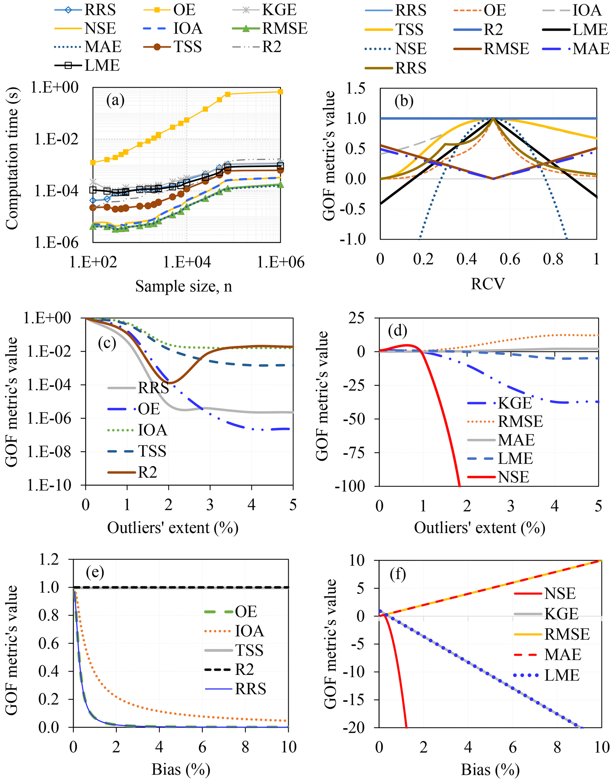
Figure 1 Comparing GOF metrics based on (a) computational load, (b) RCV, (c–d) outliers' extent, and (e–f) model bias.

3.2 Application of HMSV and NAM

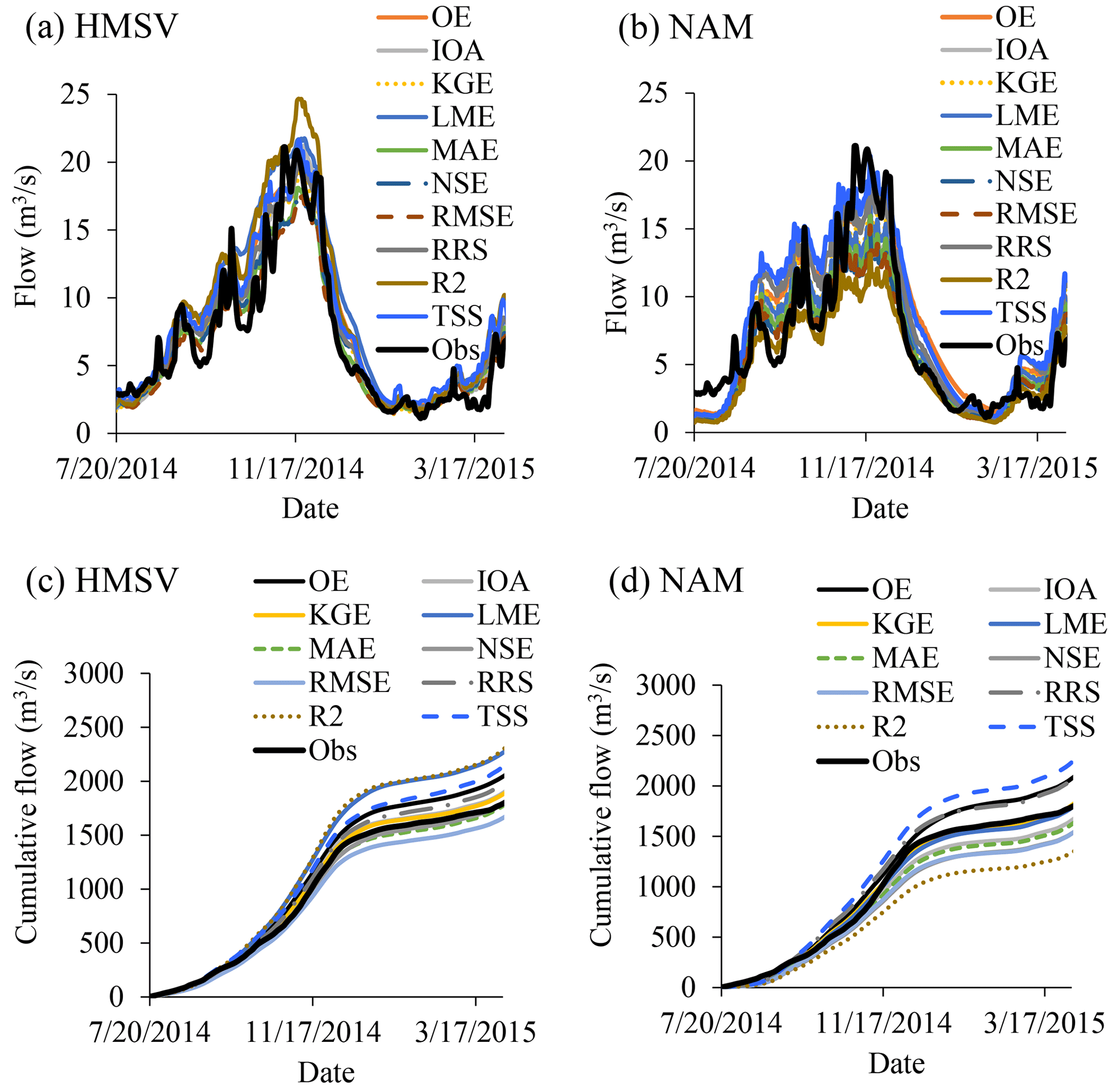
Figure 2 shows impact of the choice of an efficiency criterion on the modelled output. Modelled series based on various efficiency criteria resonated with observations to various extents (Fig. 2a–b). Considering HMSV (Fig. 2a), observed flow was more over-estimated by the modelled results based on R² than those obtained using other objective functions. However, modelled outputs based on RMSE exhibited the largest under-estimation compared with results from other objective functions. While considering NAM (Fig. 2b), results based on calibration using almost all selected objective functions resulted into under-estimation of the maximum observed flow. The largest and smallest under-estimation was from results based on R² and TSS, respectively.

The water balance closure was noted to depend on the selected efficiency criterion. The dissimilarity in the extent of spread of the right tails of the cumulative flow generated by HMSV and that of NAM was due to the difference in the structures of the models (Fig. 2c–d). One key area in which these hydrological models tended to differ was in reproducing observed peak flows.

Figure 2 Observed (Obs) flow versus outputs of (a, c) HMSV and (b, d) NAM.

3.3 Discussion

Known sources of uncertainty in hydrological models include model structure, input data errors, parameters, and calibration methods. However, this study, based on results from Figs. 1 and 2, showed that the choice of an objective function is another sub-source of calibration-related uncertainty. In other words, the choice of an efficiency criterion influences judgment of a model's quality (Onyutha, 2016). Expressly, the choice of an objective function influences the outputs of a model. Thus, it is important for a modeller to know their pros and cons of the various GOF metrics or objective functions.

3.3.1 Coefficient of determination (R²)

The metric R² (Eq. 1) varies from 0 to 1. Advantages of R² are that: it is popular, can be computed fast, and R² does not have the interpretability limitations. Interpretation of R² is straightforward in terms of the percentage of the variability explained by the model. Furthermore, R² is suitable for variables which are linearly related when there is no bias. There are several disadvantages of R². It does not quantify bias (Onyutha, 2022) and can be sensitive to outliers in the sample. It provides invalid results when the data has measurement errors (Cheng et al., 2014). There are several common misunderstandings on the use of R²; thus, the use and interpretation of R² is confusing (Alexander et al., 2015). The metric R² can be low and high for an accurate and imperfect model, respectively (Onyutha, 2022). The most commonly used R² formula or the version based on correlation is unsuitable for analysis of relationships which are not linear. It yields the same value when we regress X on Y and vice versa (Onyutha, 2022) thereby invalidating the terming of R² as coefficient of determination. Finally, R² lacks justification for its use as a descriptive statistic (Cameron, 1993).

3.3.2 Revised R-squared (RRS)

The metric RRS (Eq. 2) (Onyutha, 2022) varies from 0 to 1 and it has a number of advantages. Its computation is fast. We get different values in the two cases when regressing X on Y and vice versa (unlike R²). Furthermore, RRS does not have interpretability limitations (Onyutha, 2022). The metric RRS indicates the amount of the total variance in observations explained by the model. A modeller can use RRS to evaluate model performance in terms of bias, correlation and variability (Onyutha, 2022). The formula for RRS does not comprise direct squaring of the error term, an aspect responsible for making other metrics (such as NSE) sensitive to large model errors. The main disadvantage of RRS is that it assumes linear relationship between X on Y.

3.3.3 Index of agreement (IOA)

The metric IOA (Eq. 3) (Willmot, 1981) ranges from 0 to 1 and the advantages of IOA are that it is widely applied and can be computed fast. The limits of the IOA do not have the interpretability limitations. Furthermore, IOA can detect additive differences in the means and variances of X and Y (Moriasi et al., 2015). The disadvantages of IOA are that it can yield high values even for poorly fit model (Krause et al., 2005; Onyutha, 2022). It is sensitive to extreme values in the sample. Furthermore, it lacks physical meaning since it does not have unit. In other words, the IOA values between zero and one are difficult to interpret.

3.3.4 Nash Sutcliffe efficiency (NSE)

The metric NSE (Eq. 4) (Nash and Sutcliffe, 1970) yields values which range from −∞ to 1 and the advantages of NSE are that it is simple and popular. Its computation can be fast. Values of NSE in the two cases when we regress X on Y and vice versa are different (unlike R²). The metric NSE has several disadvantages. It has interpretability limitation compared to other metrics which vary from zero to one (Onyutha, 2022). Furthermore, NSE lacks physical meaning since it does not have a unit. Values between the limits −∞ and 1 are difficult to interpret. The metric NSE can be sensitive to outliers. The sampling uncertainty in NSE estimator is substantial (Clark et al., 2021). The reliance of NSE on mean of observations leads to exaggerated model efficiency when analysing highly seasonal river flow (Gupta et al., 2009). The metric NSE also does not indicate bias (Jackson et al., 2019) and it is not suitable for single-event simulations since it can be inadequate in quantifying differences in the time and magnitude of peak flows (Jackson et al., 2019).

3.3.5 Kling Gupta efficiency (KGE)

The metric KGE (Eq. 5) (Gupta et al., 2009) varies from −∞ to 1 and it has a number of advantages. It is becoming popular. It considers correlation, variability, and bias measures. It takes little time to be computed. The value of KGE in the two cases when we regress X on Y and vice versa are different (unlike R²). On the other hand, there are many disadvantages of KGE. It varies from −∞ to 1 and this engenders interpretability limitations compared to other metrics which vary from zero to one (Onyutha, 2022). A model's improvement starts from KGE equal to −0.41 even if the KGE values are still negative (Knoben et al., 2019). It can be sensitive to outliers. The sampling uncertainty of KGE is substantial (Clark et al., 2021). The metric KGE assumes linear relationships among variables and it can be inadequate in evaluating model performance when this assumption is violated. Furthermore, KGE assumes that the data is normally distributed and has no outliers; thus, non-normal distribution and presence of outliers all affect the metric. While optimizing KGE, the means of the simulation or values which under-estimate $\overline{X}$, especially in the high flows will tend to be favourably selected (Liu, 2020). The metric KGE lacks physical meaning since it does not have unit. Values between the limits −∞ to 1 are difficult to interpret (not as it is clear for the values of R²).

3.3.6 Hydrological model skill score

The metric OE (Eq. 6) (Onyutha, 2022) varies from 0 to 1 and its advantages are that it does not assume linear relationship among variables. The values of OE in the two cases when we regress X on Y and vice versa are different (unlike R²). The metric OE allows model performance evaluation in terms of bias, correlation and variability (Onyutha, 2022). It does not involve direct squaring of the error term, an aspect responsible for making other metrics such as NSE sensitive to large model residuals. Like other metrics, OE has a few disadvantages. It is slightly computationally slower than other metrics such as NSE. As mentioned before, the component of OE which slightly increases the computational time is the distance correlation.

3.3.7 Liu mean efficiency (LME)

The metric LME (Eq. 7) (Liu, 2020) varies from −∞ to 1. Its advantages are that it can be computed fast. It considers correlation, variability, and bias measures. The metric LME has a number of disadvantages. It assumes linear relationship. Furthermore, it is characterized by underdetermined solutions mainly approaching the excessive flow variation (Lee and Choi, 2022). Thus, the maximum potential LME can be characterized by an infinite number solutions (Lee and Choi, 2022). The variation of LME from −∞ to 1 brings about the interpretability limitations compared to other metrics which vary from 0 to 1. Like a few other metrics, LME lacks physical meaning since it does not have a unit. Values other than one are difficult to interpret. The sampling uncertainty of LME could be substantial just like that of NSE or KGE (following the methodology of Clark et al., 2021).

3.3.8 Taylor skill score (TSS)

The metric TSS (Eq. 8) (Taylor, 2001) varies from 0 to 1. The advantages of TSS are that it is popular and can be computed fast. Limits of TSS are straightforward to interpret. However, TSS has are a number of disadvantages. It does not quantify bias. It can yield high values even for poorly fit model (Onyutha, 2022). It can also be affected by the presence of outliers in the data. The formula for TSS has a term which requires case-specific calibration to determine the maximum possible correlation attainable. Furthermore, the metric TSS assumes linear relationship. TSS also lacks physical meaning since it does not have a unit. Values between zero and one are difficult to interpret.

3.3.9 Root mean squared error (RMSE)

The metric RMSE (Eq. 9) varies from 0 to +∞ and it has several advantages. It has the same unit as the variable being modelled; thus, easy to interpret given the physical meaning. It is popular, simple and can be computed fast. The main disadvantages of RMSE are that its values remain the same in the two cases when we regress X and Y and vice versa (like that of R²). The metric RMSE can be affected by the presence of outliers in the data.

3.3.10 Mean absolute error (MAE)

The metric MAE (Eq. 10) varies from 0 to +∞. Its advantages are that it is simple and can be computed fast. It has the same unit as the variable being modelled; thus, easy to interpret given its physical meaning. There are a few disadvantages of MAE. The two cases of regressing X on Y and vice versa lead to the same value of the metric MAE. Furthermore, MAE can be dominated by even one outlier or large error.

4 Conclusions

The pros and cons of the various efficiency criteria or objective functions presented in this study highlight the need to understand the impact of each efficiency criterion on model performance assessment (or the effect of the choice of an objective function on model calibration results) before making hydrological predictions. Several sources of uncertainty in hydrological models are known including model structure, input data errors, parameters, and calibration methods. However, this study showed that the choice of an objective function for calibrating a model is also another sub-source of uncertainty related to model calibration. Therefore, a modeller should make use of several efficiency criteria to judge the quality of a model. Finally, the modeller should obtain an ensemble of modelled series using results based on various (i) objective functions used individually to calibrate a model (ii) calibration methods, and (iii) hydrological models.