the Creative Commons Attribution 4.0 License.
the Creative Commons Attribution 4.0 License.
 | 16 Sep 2020
Ensemble flood simulation for the typical catchment in humid climatic zone by using multiple hydrological models
Jie Wang
Jianyun Zhang
Xiaomeng Song
Xiaoying Yang
Yueyang Wang
A good performance of hydrological model for flood simulation is of critical importance for flood forecasting. Taking Yandu River catchment, as the study area, three hydrological models (i.e. Xin'anjiang model, TOPMODEL, artificial neural network model) and a multi-model ensemble simulation method (i.e. entropy-based method) were applied to simulate the hydrological processes of 30 flood events occurring in 1981–1987. The performance of the ensemble members and multi-model ensemble simulation method was evaluated by comparing indicators of Nash-Efficiency coefficient, errors in root mean square, peak occurrence time, and relative errors of flood peak discharge, event runoff depth. Results show that the three hydrological models perform well for hydrological simulation of all 30 storm floods with Nash and Sutcliffe Efficiency coefficient of above 0.75 and relative error of less than 10 %. However, different model exhibits a difference in simulation errors of peak discharge and peak occurrence time. For example, BP model has the smallest error of 3.78 % for peak discharge simulation while that of Xin'anjiang model and TOPMODEL are 20.9 % and 24.7 % respectively. The entropy-based ensemble simulation method improved flood simulation accuracy to some extent for all evaluation criteria comparing to the three hydrological models. It is feasible to apply entropy-based ensemble approach for improving accuracy of flood forecasting in humid regions of China.
- Article
(5344 KB) - Full-text XML
- BibTeX
- EndNote


In the context of global warming, the probability and intensity of extreme precipitation are increasing (IPCC, 2014), which further aggravates the risk of flood disasters. It is therefore critical to improve flood forecasting technologies (Pitt, 2007). Hydrological modeling has been one of the commonly used tools of flood forecasting (Werner, 2005; Song and Kong, 2010). Tens of hydrological models with different structures have been successfully developed and applied globally during the past decades. Bao (2009) considered the 1950s as an important time node to divide hydrological model development into two stages: experience-based stage and model study stage. At the former stage, statistical methods are used to analyze long-term observation records to reveal the relationships between hydrological elements and the change regular, such as unit hydrograph method (Lin, 2003), corresponding stage/discharge method (Rui, 2004) and so on. The latter one produces with the development of theoretical technologies including computer technology, 3S technology, and geographic information systems, such as Xin'anjiang (XAJ), Shanbei model, Mixed Runoff yield model in China (Zhao, 1984), SAC (Burnash, 1995) and SSARR models (Rockwood, 1968) in the US, Tank model (Sugawara, 1972) in Japan, CLS model in Italy (Craft et al., 1996), etc.
At the same time, models are divided into different types according to various criteria. Yang divides flood forecasting technology into five genres: black box genre, concept genre, residual genre, filtering genre and statistical genre (Yang, 1996). However, difference exists more or less among these models, such as model structure, model type, parameters, generalization methods and so on, causing simulation results to perform variously (Vrugt et al., 2006). While it is possible for one model to poorly simulate individual flood event, it is rare for multiple models to all yield poor performance since the deficiency of certain model may be made up by other models (Roulin, 2007). This idea fits well with the concept of multi-model ensemble. This concept was first proposed in the economic and meteorological fields in the 1960s. It refers to the use of multiple means or methods to obtain the forecast value of certain factor, and then the various forecast values are used to calculate the optimal forecasting scheme. Bates and Granger (1969), Epstein (1969) and Leith (1974), respectively, are considered to be the first to propose ensemble ideas in the economic and meteorological fields. Since then, some scholars have specialized in ensemble forecasting of meteorology. For example, Andrew et al. proposed a Bayesian ensemble method in several common circulation models (GCM) for seasonal precipitation ensemble forecasting in 2003 (Andrew, 2003). Takemasa and Masaru (2011) developed the WRF-LETKF system to forecast precipitation by combining a mesoscale numerical weather prediction model (WRF) and a filtering algorithm (LETKF). Mudasser et al. (2014) used 12 different weather models to simulate precipitation in the rainy season in New Zealand and found that the choice of ensemble method was more important than the number of ensemble members to affect simulation accuracy.
In view of the successful application of ensemble methods in meteorology, hydrologists have tried to introduce this method into flood forecasting (Balint et al., 2006). Cloke and Pappenberger (2009) proposed that Ensemble Forecasting System (EPS) in flood forecasting, which is based on the Monte Carlo structure, consisted of control prediction and disturbance prediction. Up till now, scholars have applied different ensemble methods to further improve the flood forecasting scheme. For example, Jasper et al. (2002) forecasted the inflow of Lake Maggiore using five models ensemble. Davolio (2008) forecasted floods in northern Italy by using six different rainfall-runoff models. Diks and Vrugt (2010) and Arsenault et al. (2005) used a variety of ensemble methods to simulate runoff processes in different catchments in the United States, and both found that the Granger-Ramanathan ensemble method had the highest accuracy. Arsenault et al. (2017) improved the traditional ensemble method and proposed a new idea combining multi-inputs and multi-model ensemble. They used 12 ensemble members combined with three hydrological models and four climate data, to simulate the runoff process in 424 catchments in the United States. The results show that 70 % of the catchments have greatly improved the forecasting accuracy through the ensemble method.
Flood forecasting scheme is different for different climate zone due to different hydrological characteristics (Hamill et al., 2004; Guan et al., 2018). Yangtze River is the first largest river in China in terms of its drainage area and river length. Effective flood forecasting is of critical importance for flood control of this river basin. However, there are rare studies of flood forecasting by using ensemble method of multiple models, particularly for tributaries of the Yangtze River. In this paper, taking Yandu River catchment, a tributary of upper Yangtze River, as a study case, three hydrological models (e.g. Xin'anjiang model, TOPMODEL, artificial neural network model) were used to simulate flood events in 1981–1987. Then the entropy-based method is used to ensemble multiple models so as to improve the forecasting scheme and the accuracy of flood forecasting, which can provide preliminary data support for the further promotion of hydrological models ensemble application research. The remainder of this paper is organized as follows: Sect. 2 contains a brief description of the study area, three hydrological models, the ensemble method and the evaluation criteria. The results of individual model and multi-model ensemble are described in Sects. 3 and 4 gives conclusions of the study.
2.1 Study area
The Yandu River catchment is located in Badong County, Hubei Province, China, in the upper tributary of the Yangtze River, with a catchment area of 601 km2. The terrain in the catchment is mostly mountainous and covered with dense vegetation of forest and grass. The catchment situates in typical monsoon climate zone with mean annual temperature of 11.5 ∘C, and mean annual precipitation of about 1650 mm. The flood season mostly starts from May and ends in September. There are five rain stations in the catchment. The outlet hydrometric station of Yandu station was established in 1958. The river system and locations of rain gauges and hydrometric station are shown in Fig. 1. Thirty flood events in 1981–1987 were used to evaluate performance of hydrological model for flood simulation. Rainfall and discharge data with temporal resolution of 1 h were collected from Hydrological Yearbook published by Hydrology Bureau (Ministry of Water Resources of China, 1981–1987).
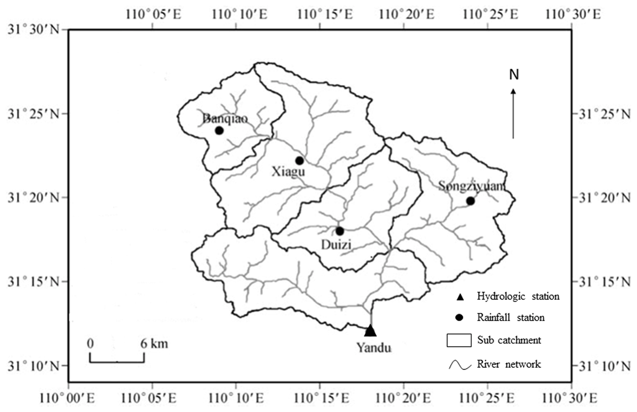
Figure 1River networks and observational station distribution.
2.2 Hydrological models
2.2.1 XAJ model
Xin'anjiang model (XAJ) is a conceptual rainfall-runoff model developed by HoHai University (Zhao, 1984). The XAJ model is based on mechanism of saturation excess. The model is mainly composed of four parts, namely runoff yield, evapotranspiration, water source partition and confluence. For flood simulation, hourly rainfall series are needed to drive XAJ model. The model structure and parameters are shown in Fig. 2.
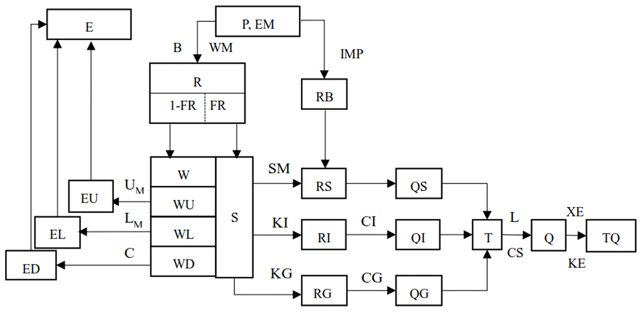
Figure 2Framework of the Xin'anjiang Model. Note: K: Reduction coefficient of evaporation; IMP: Impervious area proportion; B: Exponent of storage capacity curve; WM: Average water storage capacity in the catchment; WUM: Storage capacity of the upper layer; WLM: Storage capacity of the lower layer; C: Evapotranspiration coefficient of deeper layer; SM: Storage capacity of free water; EX: Exponent of free water storage capacity curve; KG: Outflow coefficient of free water storage to groundwater; KI: Outflow coefficient of free water storage to interflow; CG: Regression coefficient of groundwater storage; CS: Regression coefficient of surface runoff; CI: Regression coefficient of interflow storage; L: Coefficient of hysteresis calculation; XE: Muskingum parameter; KE: Muskingum parameter.
2.2.2 TOPMODEL
TOPMODEL is a semi-distributed watershed hydrological model proposed by Beven and Kirkby (Xu, 2009). The model is based on the concept of variable flow generation with consideration of catchment topographical features, soil texture, etc. The model divides soil layer into three aquifer zones, vegetation root zone, unsaturated soil zone, and saturated soil zone. The inputs of TOPMODEL not only include rainfall series, but also include catchment topographic index ln(α∕tan β). Digital Elevation Model (DEM) data is therefore needed for the model application. Total runoff is the sum of interflow and saturated slope flow. The conceptual framework of the TOPMODEL is shown in Fig. 3. There are five parameters in TOPMODEL need to calibrate.

2.2.3 BP model
The BP model is a multi-layered feedforward neural network with a strong self-learning ability. It can transmit corrected errors in reverse order (Zhao, 1996). Its hierarchy includes the input layer, the hidden layer, and the output layer. This paper uses a three-layer BP model with only one hidden layer. The structure of the constructed BP model is 8-17-1, shown in Fig. 4. It means BP model has 8 inputs, including data from 5 precipitation station data and discharge data for the first three moments. The only output of the model is the discharge at the corresponding time of the basin outlet. The intermediate layer is connected to the input and output and is calculated as 17 layers by the empirical formula, representing the complexity of the established model.
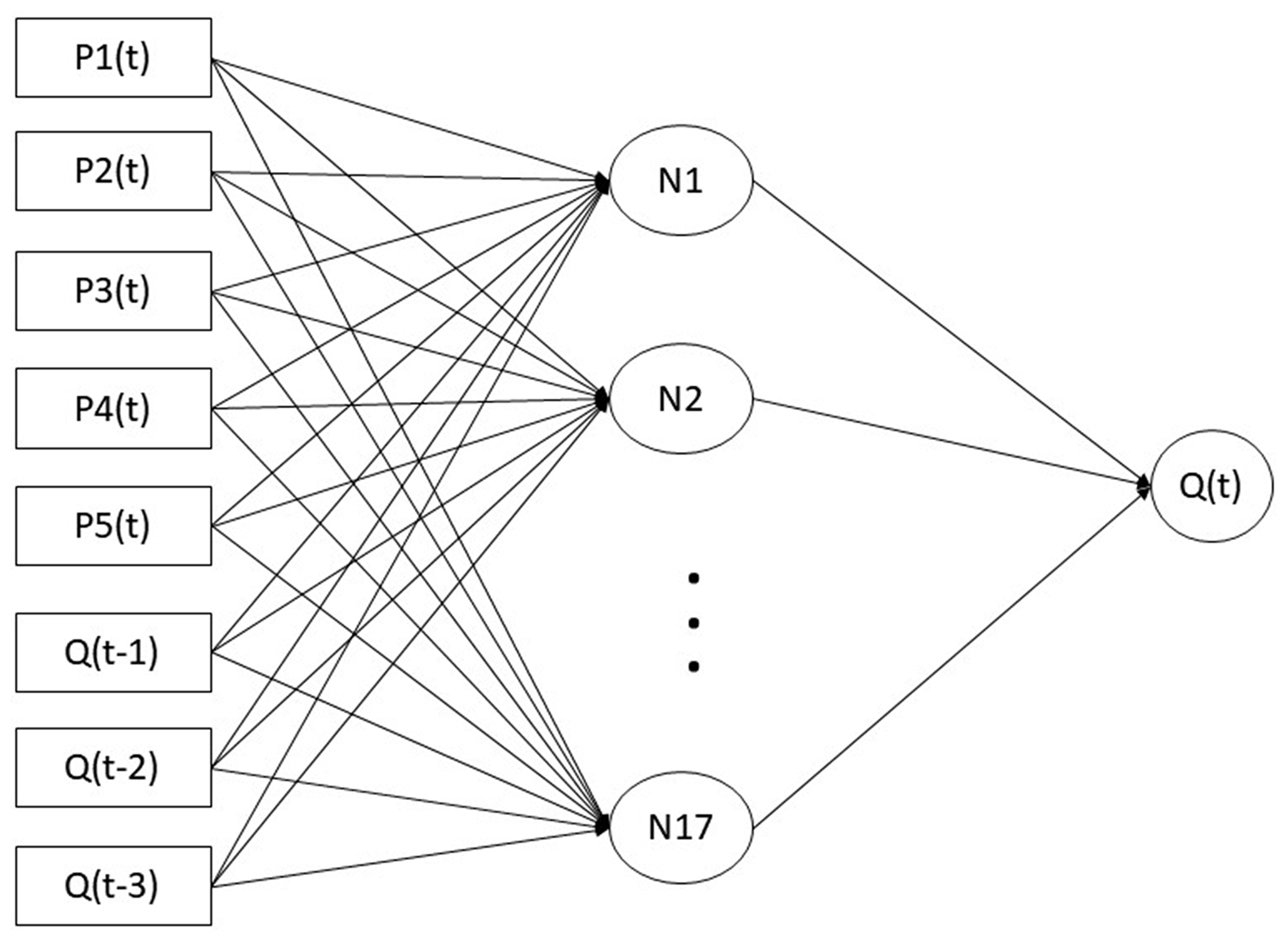
Figure 4BP model flowchart. Note: P1(t), P2(t), P3(t), P4(t), P5(t): five precipitation station data; Q(t−1), Q(t−2), Q(t−3): discharge data for the first three moments; N1–N17: the intermediate layer nodes; Q(t): discharge at the corresponding time of the basin outlet.
2.3 Entropy-based ensemble method
In ensemble methods, it is important to identify the weight coefficients. The basic idea of the entropy method is that the variation of the error between the simulated and observed results is inversely proportional to the weight coefficient.
Firstly, calculate the errors between the simulated and observed results and normalize the errors:
Secondly, calculate the entropy value of the relative error in the model simulation:
Thirdly, calculate the variation index and weight coefficient:
Assume at, t=1, 2, 3, …, m is the sequence of simulation objects and there are n kinds of single models to simulate, then the simulation value of the method i at time t is ait, i=1, 2, …, n. Where Eit and Bit represent the relative errors and normalized errors of the method i at the time t, at represent the observed value at time t, while Hi, Di, Qi mean the entropy value, variation index and weight coefficient of model i.
2.4 Evaluation criteria
Five evaluation criteria of Nash and Sutcliffe efficiency coefficient (so called Nash-Efficiency Coefficient, NEC), errors in root mean square (RSME), error in time to flood peak (ETFP), relative error in flood peak discharge (REFPD) and relative error in event runoff depth (REERD), were selected to evaluate performance of hydrological model for flood simulation. Details about the five evaluation criteria could be found in manual guideline of flood forecasting issued by the Ministry of Water Resources of the People's Republic of China (2008). Good performance of hydrological model for flood simulation will have NEC approaching to 1 and RSME, ETFP, REFPD, and REERD being close to 0.
3.1 Flood characteristics
Being influenced by Asian monsoon climate, floods in the Yandu River mostly occur in period from May to September with 2–19 d duration. Statistical results of the selected 30 floods indicated that flood peak discharge ranges from 300 to 1200 m3 s−1 while the corresponding event rainfall varies in range of 35.7–331.7 mm. The hydrograph of flood is highly influenced by the spatiotemporal distribution pattern of rainfall. 56.7 % of flood events have multiple peaks. Flood runoff depth against rainfall in 30 flood events were plotted in Fig. 5.
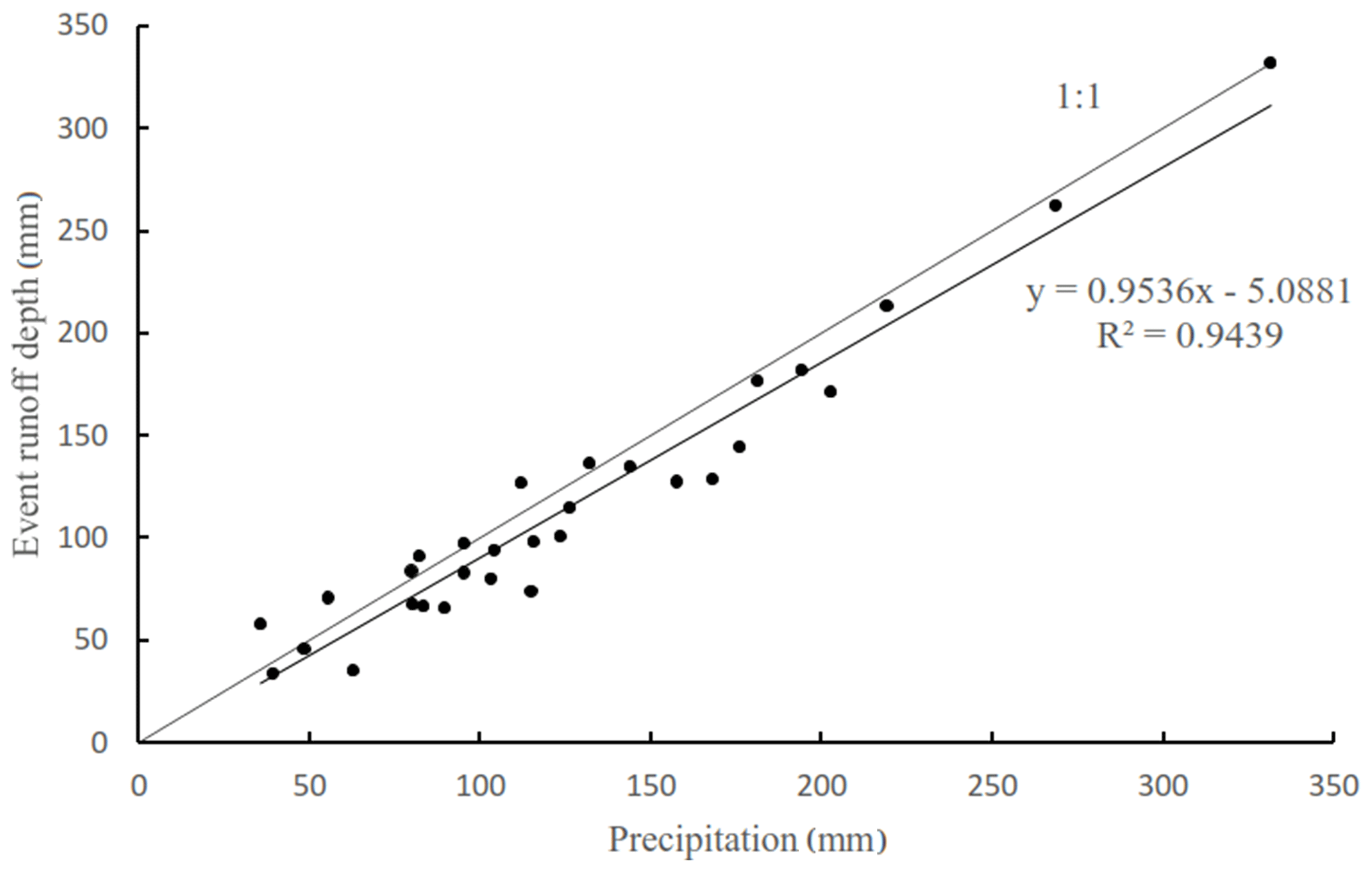
According to the trend line of the precipitation-runoff (P-R) point group of 30 floods, the slope is 0.95, which is very close to the 1:1 line and is below the 1:1 line. The slope represents the runoff coefficient here and its value is close to 1, indicating that the loss of the event flood is relatively small overall. This indicates that the study area is humid and antecedent soil moisture is abundant. The P-R relationship of about 7 floods falls above the 1:1 line. The runoff coefficient of seven floods is more than 1 due to the influence by previous rainfall. Previous runoff had not completely regressed before the next flood occurred, causing higher runoff than rainfall.
Table 1The results of parameters calibration in XAJ hourly model.
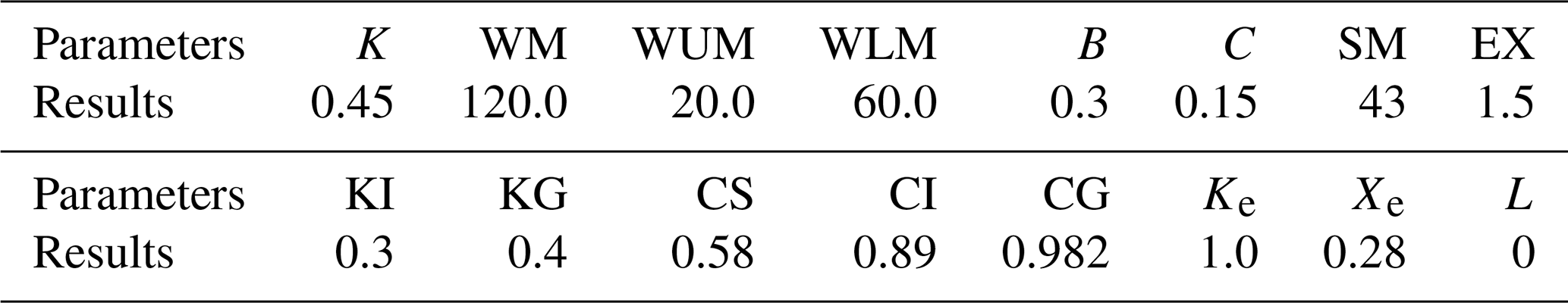
Note: K: Reduction coefficient of evaporation; IMP: Impervious area proportion; B: Exponent of storage capacity curve; WM: Average water storage capacity in the catchment; WUM: Storage capacity of the upper layer; WLM: Storage capacity of the lower layer; C: Evapotranspiration coefficient of deeper layer; SM: Storage capacity of free water; EX: Exponent of free water storage capacity curve; KG: Outflow coefficient of free water storage to groundwater; KI: Outflow coefficient of free water storage to interflow; CG: Regression coefficient of groundwater storage; CS: Regression coefficient of surface runoff; CI: Regression coefficient of interflow storage; L: Coefficient of hysteresis calculation; XE: Muskingum parameter; KE: Muskingum parameter.
Table 2The calibrated parameters of TOPMODEL.

Note: m: Rate parameter of soil infiltration intensity decreasing exponentially; ln(T0): Natural logarithm of soil effective conductivity reaching saturation; SRmax: Maximum water storage capacity in root zone; SRinit: Volume of initial water shortage; ChVel: Effective surface convergence speed.
3.2 Model calibration and flood simulation
Three individual models were used to simulate hourly flow. Experience method and manual-trail-error method were used for parameter calibration in the XAJ model, and the results were shown in Table 1. As for the TOPMODEL, topographic index of Yandu River catchment was calculated with ArcGIS (Fig. 6) and then used as model inputs. Its parameters were calibrated by manual-trial-error method (Table 2). In BP model, automatic calibration method (Levenberg-Marquardt method, Levenberg, 1944; Marquardt, 1963) was used for model parameter calibration, where 153 weights and 18 thresholds need to be determined. Due to the length of the article, BP model parameters are not shown in this paper.
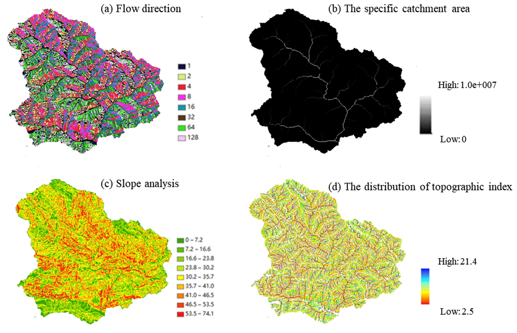
Figure 6Topographic index calculation process.
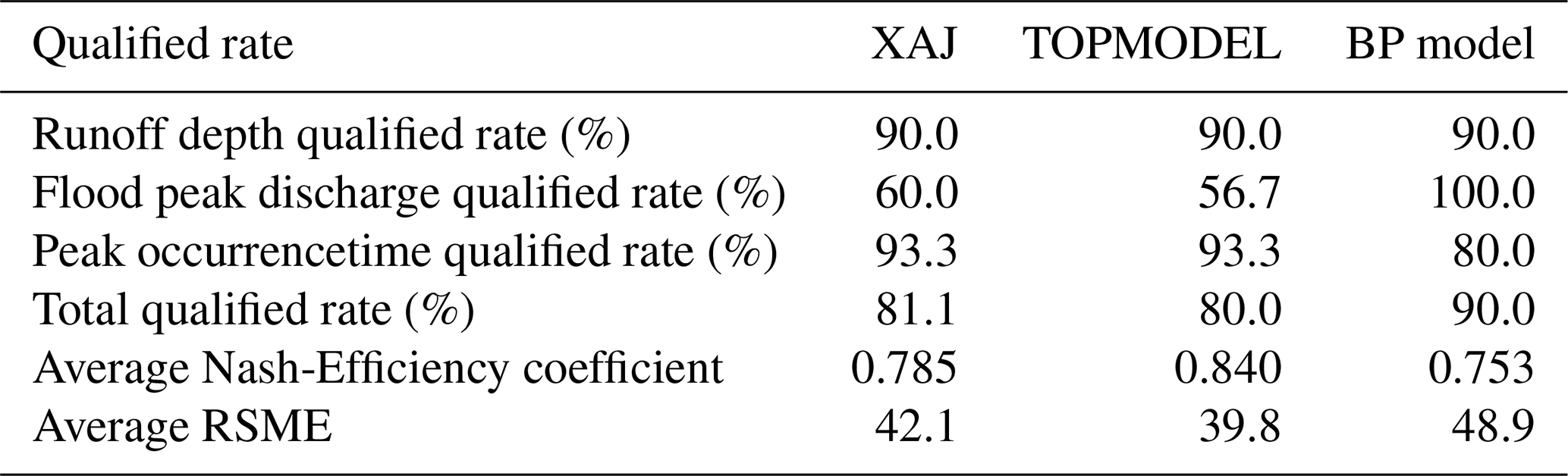
Evaluation statistics of the three models are shown in Table 3. There are differences in the simulation results among the three models. Combined with the multi-objective evaluation results, the BP model based on the self-memory pattern has the highest total qualified rate (90.0 %), but each model shows a large difference under different evaluation conditions. XAJ model has the highest peak occurrence time qualified rate (93.3 %); BP model has the highest qualified rate at the flood peak discharge (100 %); TOPMODEL has the highest runoff depth qualified rate (90 %), the highest Nash-Efficiency coefficient (0.840) and the lowest average RSME (39.8).
Table 3Comparison of results derived by single hydrological model for flood simulation.
3.3 Ensemble flood simulation with multiple models
The entropy method was used to calculate the weight coefficients of the three models. In simulating different flood, each model is assigned with different weight coefficient as shown in Table 4. For the 30 floods, the average weight coefficients of the XAJ model, TOPMODEL and BP model are 0.347, 0.299, and 0.354, respectively. This indicates that the three models contribute differently to the ensemble results. The order of the three models is BP model, XAJ model, and TOPMODEL based on its weight from high to low. This indicates that, to some extent, simulation results of the BP model are better.
Table 4Weight coefficients assigned to the three models based on the entropy method.

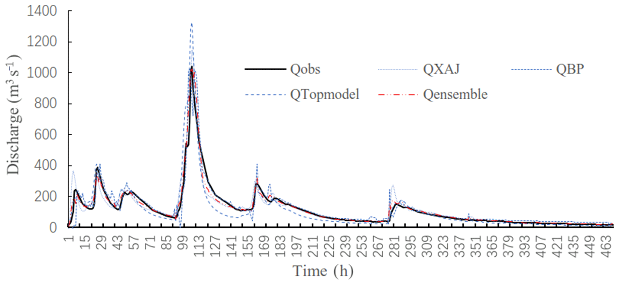
Figure 7 compared the hydrograph of the 820 716 flood yielded by the three individual models and the ensemble. As seen from the figure, the ensemble flood hydrograph is closer to the observed flood hydrograph than all those yielded by single models.
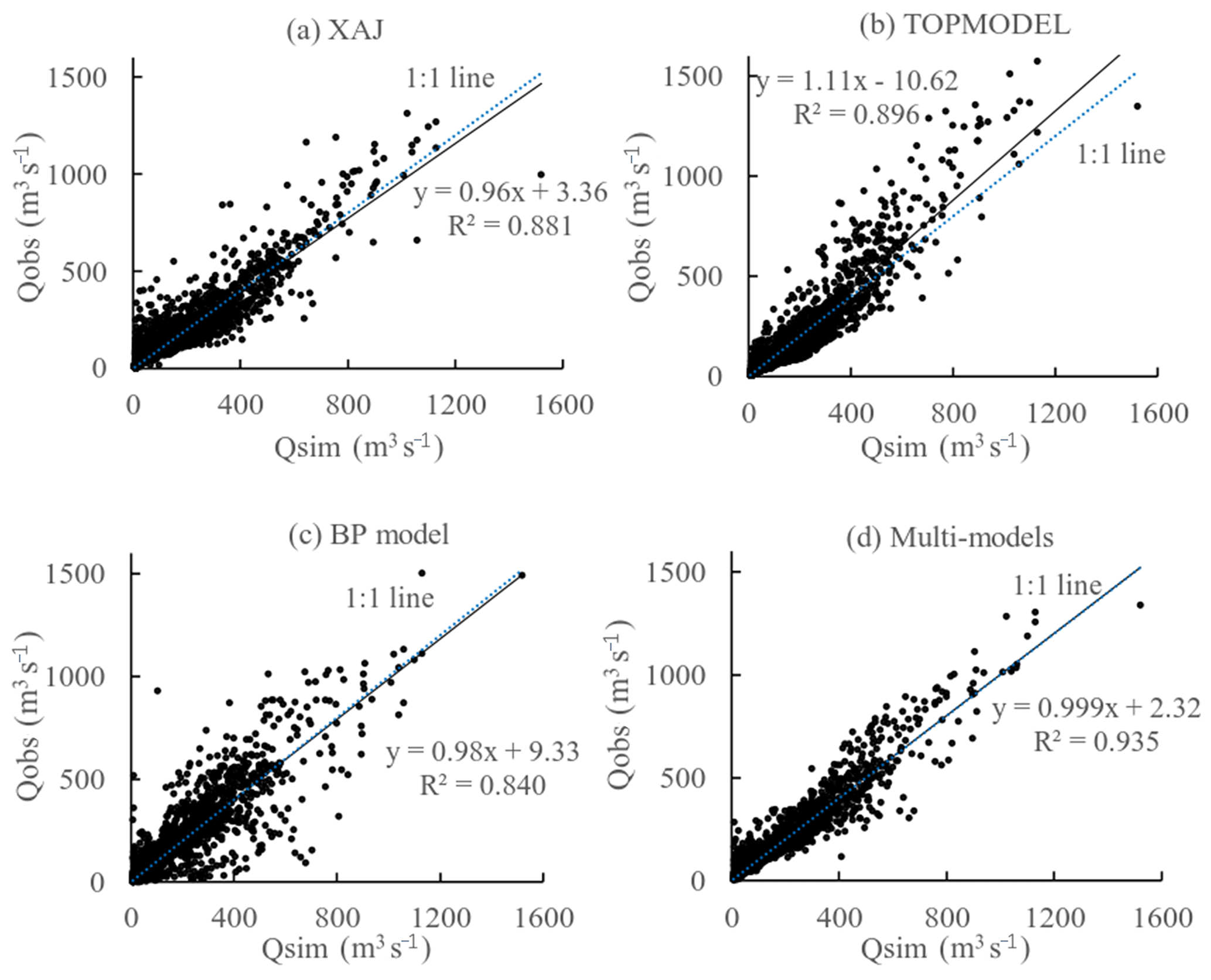
Figure 8 gives the scatterplots between observed and simulated flood discharge by three single models and the multi-model ensemble. With R2 greater than 0.8, simulated discharge by all three models has a good linear relationship with observations. The trend lines of the XAJ model and BP model are close to the 1:1 line, indicating their better discharge simulation performance. The trend line of the TOPMODEL is above the 1:1 line, indicating its simulated values tend to be higher than observed values. Higher than all three single models, the R2 value of the multi-model ensemble reaches 0.935.
Table 5Statistics of evaluation indexes.
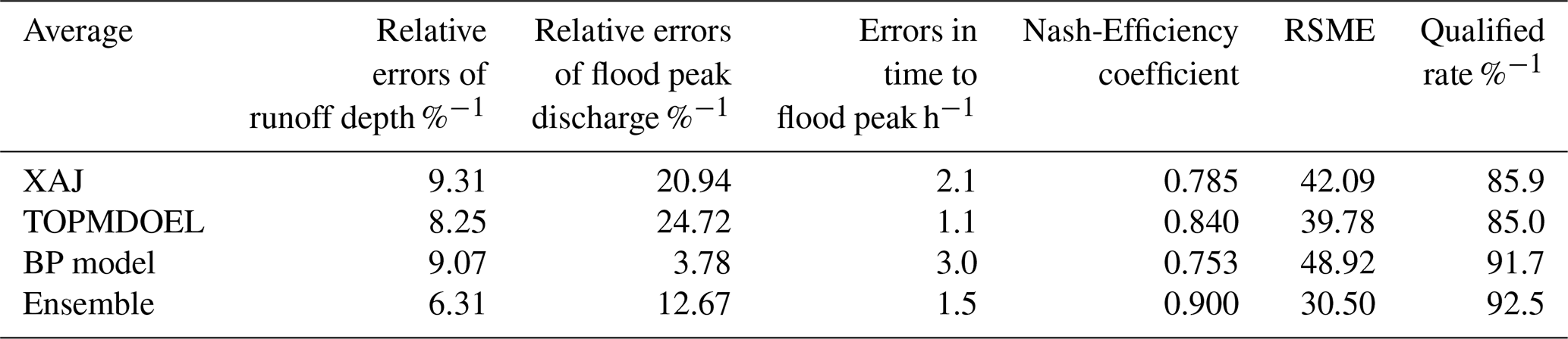
Note: (1) The bold font in the table indicates the item whose ensemble result reduces the accuracy of the single model result. (2) The error average value in the table is the average value of the absolute value of the relative error of each field.
The average results of six indicators in the single model and the multi-model ensemble were compared, as shown in Table 5. It can be seen that compared with the single model, the multi-model ensemble method effectively reduces various errors and improves the Nash-Efficiency coefficient and the qualified rate. Among them, the ensemble results are better than the single model except the flood peak discharge and peak occurrence time. Although the relative errors of flood peak discharge is larger than that of BP model, relative to XAJ model and TOPMODEL is significantly reduced. The ensemble peak error is higher than TOPMODEL, but it is lower than the XAJ model and the BP model. Only two items are lower than the ensemble results, and the overall improvement is more significant.

In order to more intuitively understand the distribution of the improvement degree of the multi-model ensemble results relative to the single model, the box line diagrams of the improvement degree in each evaluation objective function were drawn, as shown in Fig. 9. As seen from Fig. 9a, the median, mean and interquartile range of the boxplots are similar, indicating that the ensemble plays a similar role in reducing the relative error of the event runoff depth for the three models. For the peak discharge, the XAJ model and the TOPMODEL box are basically in the positive range, while the BP model box is in the negative range, indicating that the ensemble has significant improvements for the first two models (Fig. 9b). The ensemble has the greatest improvement on TOPMODEL, with the box basically above the x-axis. However, the peak discharge accuracy of the BP model is decreased after multi-model ensemble. Moreover, for the peak time (Fig. 9c), the error in time to flood peak of BP is reduced the most, with an average decrease of 1 h. The XAJ model has a single flood error reduced by 24 h, which is the model with the largest error reduction. However, the error in time to flood peak of the other floods generally increased after multi-ensemble. As for Nash-Efficiency coefficient (Fig. 9d), the BP model has the greatest improvement, and the Nash-Efficiency coefficient increases by an average of 0.14. In conclusion, after the multi-model ensemble, the models were improved to different degrees in the accuracy except the individual models and several floods.
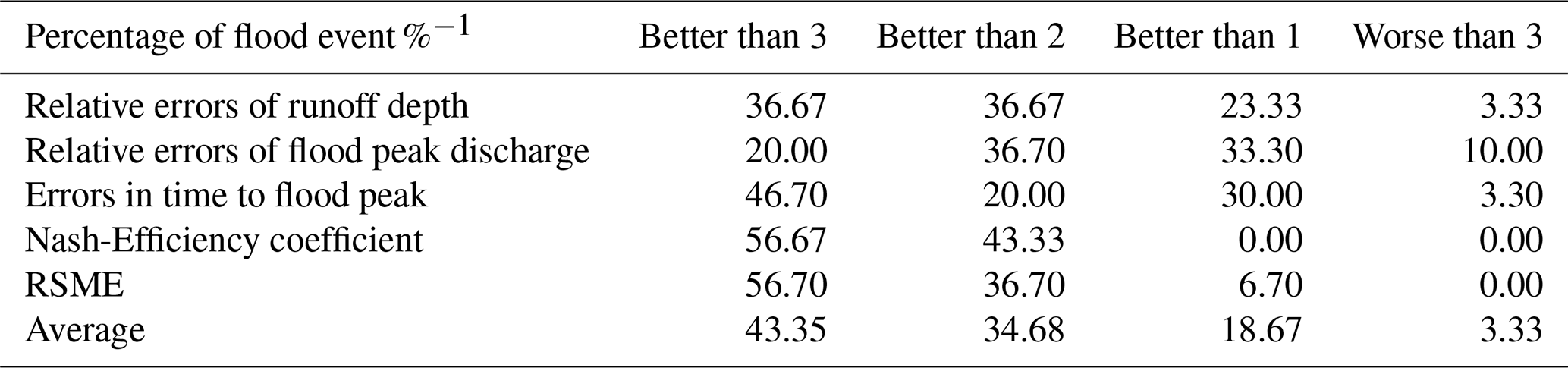
According to the improvement of the evaluation criteria above results, the number of ensemble results was count in this paper, as shown in Table 6. On the average, the multi-model ensemble performed better than all three models in simulating 43.4 % of the 30 flood events. It shows the most improvement in terms of the Nash-Efficient coefficient and RSME by yielding better results for more than 15 floods than all three single models. In addition, the multi-model ensemble givers better overall performance than two models for 34.68 % of the floods, and one model for 18.67 % of the floods. The ensemble accuracy of the event runoff depth for only one flood, the flood peak discharge for two floods, and the peak occurrence time for one flood is lower than the single model, accounting for a lower proportion. So it can be considered that the accuracy results obtained by multi-model ensemble are significantly improved compared to the single model.
3.4 Discussion
XAJ model and TOPMODEL both perform well, the manual-trial-error method was used to calibrate the parameters, which made the results of some floods relatively unsatisfactory. Because it takes into account the influencing factors such as basin topography and soil properties, TOPMODEL performs slightly better than the XAJ model. Based on a self-learning algorithm, the BP model is the best among the three models in discharge simulation. However, it is essentially a statistical model with little representation of physical mechanisms.
The purpose of ensemble method is to determine the weight and methods are various. Entropy-based ensemble method in this paper has many advantages comparing to the simple weighted average. The closer the simulated value and measured value, the larger the weight. Each flood has a set of weights, which can get the best ensemble scheme in each flood. In the future, more methods can be chosen for comparative discussion.
The central idea of this paper is to carry out flood simulation. This is the preliminary work of flood forecasting. For forecasting, it may be considered to classify the floods according to the characteristics of the floods, determine the set of weight parameters for each type, and then carry out the forecasting work, which needs further improvement and verification in the future.
The XAJ model, TOPMODEL and BP model all perform well in the simulation of floods in the Yandu River catchment. Overall, the BP model has the highest forecast qualified rate (90 %). The Nash-Efficiency coefficient, runoff depth and peak time accuracy of the XAJ model and TOPMODEL are relatively high, while the flood peak discharge accuracy of the BP model is relatively high. Taking into account the overall simulation performance, the parameter failed to take care of all flooding floods. So the simulation accuracy of few floods is not ideal.
The entropy method was used to calculate the weight coefficients of the three models in the ensemble. Comparison of five model evaluation statistics had shown that the multi-model ensemble had improved flood simulation to various degrees. On the average, the multi-model ensemble reduces the relative errors of the runoff depth by 3.9 %, the relative errors of the flood peak discharge by 1.5 %, the error in time to flood peak by 0.4 h and the RSME by 10.9. At the same time, it increases the average Nash-efficiency coefficient by 0.1. Eighty percent of the flood ensemble results are better than at least two single model results.
Data is available based on request to the corresponding authors.
JW contributed results analysis and drafting the manuscript, JZ and Guoqing Wang structured the manuscript and contributed results discussion, XS contributed methodology of the work, XY contributed analysis on results reasonability, YW contributed data collection.
The authors declare that they have no conflict of interest.
This article is part of the special issue “Hydrological processes and water security in a changing world”. It is a result of the 8th Global FRIEND–Water Conference: Hydrological Processes and Water Security in a Changing World, Beijing, China, 6–9 November 2018.
We are thankful to anonymous reviewers and editors for their helpful comments and suggestions.
This research has been supported by the National Key Research and Development Program of China (no. 2016YFA0601501), the National Natural Science Foundation of China (grant nos. 41830863, 41330854, 51879162, 51609242, 51779146, 41601025), and the State Key Laboratory of Hydrology – Water Resources and Hydraulic Engineering (grant nos. 2017490211, 2015490411)
Andrew, W. R., Upmanu, L., Stephen, E. Z., and Balaji, R.: Categorical climate forecasts through optimal combination of multiple GCM ensembles, World Water and Environmental Resources Congress, 130, 1792–1811, https://doi.org/10.1061/40685(2003)184, 2003.
Arsenault, R., Gatien, P., Renaud, B., Brissette, F., and Martel, J. L.: A comparative analysis of 9 multimodel averaging approaches in hydrological continuous streamflow simulation, J. Hydrol., 529, 754–767, https://doi.org/10.1016/j.jhydrol.2015.09.001, 2005.
Arsenault, R., Gilles, R. C., and Francois, P. B.: Improving hydrological model simulations with combined multi-Input and multimodel averaging frameworks, J. Hydrol. Eng., 22, 66–76, https://doi.org/10.1061/(ASCE)HE.1943-5584.0001489, 2017.
Balint, G., Csik, A., Bartha, P., Gauzer, B., and Bonta, I.: Application of meterological ensembles for Danube flood forecasting and warning, in: Transboundary floods: Reducing risks through flood management, edited by: Marsalek, J., Stancalie, G., and Balint, G., Springer, NATO Science Series, Dordecht, the Netherlands, 57–68, 2006.
Bao, W.: Hydrological forecasting (4th Edn.), China Water Conservancy and Hydropower Press, China, 141–142, 2009.
Bates, J. M. and Granger, C. W. J.: The combination of forecasts, Oper. Res. Aquart., 20, 451–468, 1969.
Burnash, R. J. C.: The NWS river forecast system-catchment modeling, in: Computer models of watershed hydrology, edited by: Singh, V. P., Water Resour. Publ. Am., 4, 311–366, 1995.
Cloke, H. L. and Pappenberger, F.: Ensemble flood forecasting: A review, J. Hydrol., 375, 613–626, 2009.
Craft, T. J., Launder, B. E., and Suga, K.: Development and application of a cubic eddy-viscosity model of turbulence, J. Heat Fluid Flow, 17, 108–115, https://doi.org/10.1016/0142-727X(95)00079-6, 1996.
Davolio, S., Miglietta, M. M., Diomede, T., Marsigli, C., Morgillo, A., and Moscatello, A.: A meteo-hydrological prediction system based on a multi-model approach for precipitation forecasting, Nat. Hazards Earth Syst. Sci., 8, 143–159, https://doi.org/10.5194/nhess-8-143-2008, 2008.
Diks, C. and Vrugt, J.: Comparison of point forecast accuracy of model averaging methods in hydrologic applications, Stoch. Env. Res. Risk A., 24, 809–820, https://doi.org/10.1007/s00477-010-0378-z, 2010.
Epstein, E. S.: Stochastic dynamic prediction, Tellus, 21, 739–759, https://doi.org/10.1111/j.2153-3490.1969.tb00483.x, 1969.
Guan, X., Liu, Y., Jin, J., Liu, C., Liu, Y., and Wang, G.: Hydrological variation characteristics of typical watersheds in different climate regions of China, Journal of North China University of Water Resources and Electric Power (Natural Science Edition), 39, 13–17, 2018.
Hamill, T., Whitaker, J., and Wei, X.: Ensemble reforecasting: improving medium-range forecast skill using retrospective forecasts, Mon. Weather Rev., 132, 1434–1447, 2004.
IPCC (Intergovernmental Panel on Climate Change): Climate change 2014: Synthesis report. Geneva Switzerland: Contribution of working groups I, II and III to the fifth assessment report of the intergovernmental panel on climate change, 85–88, 2014.
Jasper, K., Gurtz, J., and Lang, H.: Advanced flood forecasting in Alpine watersheds by coupling meteorological observations and forecasts with a distributed hydrological model, J. Hydrol., 267, 40–52, https://doi.org/10.1016/s0022-1694(02)00138-5,2002.
Leith, C. E.: Theoretical skill of Montre Carlo forecast, Mon. Weather Rev., 102, 409–418, 1974.
Levenberg, K.: A method for the solution of certain nonlinear problems in least squares, Q. Appl. Math.s, 2, 164–168, https://doi.org/10.1090/qam/10666, 1944.
Lin, S.: Hydrological forecasting, 2nd Edn., China Water Conservancy and Hydropower Press, Beijing, China, 58–62, 2003.
Marquardt, D. W.: An algorithm for least squares estimation of nonlinear parameters, J. Soc. Ind. Appl. Math., 11, 431–441, 1963.
Ministry of Water Resources of the People's Republic of China: Hydrological yearbook published by Hydrology Bureau, China Water Conservancy Press, China, 1981–1987.
Ministry of Water Resources of the People's Republic of China: Hydrological information forecasting specification, China Water Conservancy Press, China, 5–6, 2008.
Mudasser, M. K, Asaad, Y. S., and Brucem, W. M.: Impact of ensemble size on forecasting occurrence of rainfall using TIGGE precipitation forecasts, J. Hydrol. Eng., 19, 732–738, https://doi.org/10.1061/(ASCE)HE.1943-5584.0000864, 2014.
Pitt, M.: Learning lessons from the 2007 floods: an independent review by Sir Michael Pitt: interim report, UK, 32–33, 2007.
Rockwood, D. M.: Application of streamflow synthesis and reservoir regulation – SSARR-program to the lower Mekong River. The use of Analog and Digital Computers in Hydrolog, 377–378, https://doi.org/10.1016/0002-9378(93)90010-G, 1968.
Roulin, E.: Skill and relative economic value of medium-range hydrological ensemble predictions, Hydrol. Earth Syst. Sci., 11, 725–737, https://doi.org/10.5194/hess-11-725-2007, 2007.
Rui, X.: Hydrology principle, China Water Conservancy and Hydropower Press, China, 3–4, 2004.
Song, X. and Kong, F.: Application of Xin'anjiang model coupling with artificial neural networks, Bulletin of Soil and Water Conservation, 30, 135–138, 2010.
Sugawara, M.: Analysis method of valley discharge, Koritsu publisher, Janpan, 110–116, 1972.
Takemasa, M. and Masaru, K.: The local ensemble transform Kalman Filter with the weather research and forecasting model: experiments with real observations, Pure Appl. Geophys., 169, 321–333, https://doi.org/10.1007/s00024-011-0373-4, 2012.
Vrugt, J. A., Gupta, H. V., Nuallain, B., and Bouten, W.: Real-time data assimilation for operational ensemble streamflow forecasting, J. Hydrometeorol., 7, 548–565, https://doi.org/10.1175/JHM504.1, 2006.
Werner, M.: FEWS NL Version 1.0 – Report Q3933, Delft Hydraulics, Delft, 2005.
Xu, Z.: Hydrological models, Science Press, China, 318–340, 2009.
Yang, X.: A review of real-time flood forecasting methods, Chinese Hydrology, 65, 9–16, 1996.
Zhao, R.: Hydrological simulation – Xin'anjiang model and Shanbei model, Water Power Press, Beijing, China, 106–118, 1984.
Zhao, Z.: The Foundation and Application of Fuzzy Theory and Neural Network, Tsinghua University Press, China, 125–129, 1996.