Initial results of sediment yield measurement interpretation using a regional approach: Southern Italy case study

The theoretical TCEV (Two Component Extreme Value) distribution was applied to interpret the sediment yield datasets available in Southern Italy. The analysis is based on hydrological data collected for twelve catchments located in Calabria and Basilicata. A hierarchical approach was used to obtain a regional parent distribution which was used to determine the return time for each event. The hierarchical approach proposed in this study includes two stages. The first stage served for calibration and made it possible to estimate the parameters of the theoretical TCEV distribution. More specifically, the hypothesis of homogeneity with regard to the skewness coefficient and the coefficient of variation was verified using the datasets related to nine catchments. The second stage consisted in verifying the goodness of the theoretical distribution on three independent datasets provided by three experimental catchments not involved in the calibration. Overall results show that, even if the TCEV distribution was conceived to estimate peak flow, its concept of “double component” can be extended to predict sediment yield on a regional scale.

1 Introduction

Prediction of soil erosion and sediment yield, corresponding to a fixed return time, is necessary to adopt soil conservation strategies for reducing costs of on-site and off-site impacts in areas at risk.

In Southern Italy, high rates of soil erosion and sediment yield are well documented both on cultivated land (Porto and Walling, 2012) and in areas covered by forests (Porto et al., 2004). Over the last 60 years, predictions of sediment yield are based both on the use of traditional monitoring techniques, such as observations on experimental plots or catchments, and on different types of models that vary from empirical-parametric approaches, such as SEDD (Ferro and Porto, 2000) or revised versions of the USLE (Cinnirella et al., 1998) to more recent physically- based models, such as WEPP (Nearing et al., 1989), whose goal is to simulate both the detachment and transport of soil particles.

However, even if these models provide good estimates of long-term average values of sediment yield, they cannot make reliable predictions associated to a fixed return time especially if they are associated with extreme events.

A recent study (Porto and Callegari, 2019), carried out on three experimental catchments (W1, W2, and W3) located in Calabria (Southern Italy), demonstrated that a significant proportion of the annual sediment yield in these catchments is due to the extreme event occurred each year which produced more than 50 % of the total annual sediment yield with a very few exceptions.

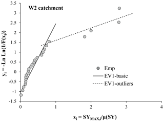
Looking at the frequency distribution of these measurements of sediment yield, the same authors showed that the empirical distribution of the normalized variable $x_i={\text{SY}}_{\mathrm{MAX},i}/\mathit{\mu }\left(\text{SY}\right)$, where SY_MAX,i. is the maximum annual value and μ(SY) is the mean annual value of the entire monitoring period, is skewed. In particular, results of observation on the catchment W2 (see Porto and Callegari, 2019) shows that two components can be identified (Fig. 1). One of them is associated with ordinary events (basic component) and a second one is characterized by extreme events (outliers component).

Figure 1 Gumbel's plot for the dataset of the normalized variable, $x_i={\text{SY}}_{\mathrm{MAX},i}/\mathit{\mu }\left(\text{SY}\right)$.

The authors concluded that the process can be represented by two Extreme Value Type 1 (EV1) independent distributions, one for each component, capable of associating each event with a corresponding return time T. The double component indicated in Fig. 1 is a well known effect when studying annual records of maximum peak flow values (see Rossi et al., 1984) and a more sophisticated approach can be used to explain it.

This approach is based on the TCEV (Two Component Extreme Value) model whose ability was well demonstrated in predicting peak flow and critical rainfall corresponding to a fixed return time (see Rossi et al., 1984; Ferro and Porto, 1999, 2006). The TCEV distribution is based on the assumption that in each historical sample of the observed variable x, one or several annual maximum values are significantly higher than the bulk of the remaining data, so that two components are clearly distinguishable.

Therefore, the theoretical CDF of the TCEV law F(x) can be expressed as a probabilistic model with four parameters derived from the product of two EV1 distributions:

$$\begin{array}{}\text{(1)}& F\left(x\right)=\exp \left[-{\mathit{\lambda }}_{\mathrm{1}}\exp \left(-{\displaystyle \frac{x}{{\mathit{\theta }}_{\mathrm{1}}}}\right)-{\mathit{\lambda }}_{\mathrm{2}}\exp \left(-{\displaystyle \frac{x}{{\mathit{\theta }}_{\mathrm{2}}}}\right)\right]\end{array}$$

where: λ₁, λ₂ are the shape parameters and represent the mean number of events which belong respectively, to the basic (component 1) and the outlying (component 2) components; and θ₁, θ₂ are the scale parameters, which represent the at-site central values of the x variable for each component.

The basic component is characterized by a high number of events and by values of x less than those corresponding to the outlying component so that λ₁≫λ₂ and θ₁≪θ₂. The main advantage of the TCEV model, if compared to the EV1 distribution, is based on the fact that the former can be used at a regional scale because their parameters (or their combination) showed to be scale invariant for large areas.

In order to apply the model at a regional scale it is useful to introduce the standardized variable $y=\left(\frac{x}{{\mathit{\theta }}_{\mathrm{1}}}\right)-{\mathit{\lambda }}_{\mathrm{1}}$ by which Eq. (1) becomes:

$$\begin{array}{}\text{(2)}& F\left(y\right)=\exp \left[-\exp (-y)-{\mathrm{\Lambda }}_{\ast }\exp \left(-{\displaystyle \frac{y}{{\mathrm{\Theta }}_{\ast }}}\right)\right]\end{array}$$

where: ${\mathrm{\Theta }}_{\ast }={\mathit{\theta }}_{\mathrm{2}}/{\mathit{\theta }}_{\mathrm{1}}$ and ${\mathrm{\Lambda }}_{\ast }={\mathit{\lambda }}_{\mathrm{2}}/{\mathit{\lambda }}_{\mathrm{1}}^{\mathrm{1}/{\mathrm{\Theta }}_{\ast }}$.

Introducing the dimensionless variable x^′, equal to the ratio between x and the mean value μ of the TCEV distribution, Eq. (2) becomes:

$$\begin{array}{}\text{(3)}& F\left(x^{\prime }\right)=\exp \left\{-{\mathit{\lambda }}_{\mathrm{1}}{\left[\exp \left(\mathit{\alpha }\right)\right]}^{-x^{\prime }}-{\mathrm{\Lambda }}_{\ast }{\mathit{\lambda }}_{\mathrm{1}}^{\mathrm{1}/{\mathrm{\Theta }}_{\ast }}{\left[\exp \left({\displaystyle \frac{\mathit{\alpha }}{{\mathrm{\Theta }}_{\ast }}}\right)\right]}^{-x^{\prime }}\right\}\end{array}$$

named growth curve, in which:

$$\begin{array}{}\text{(4)}& \mathit{\alpha }={\displaystyle \frac{\mathit{\mu }}{{\mathit{\theta }}_{\mathrm{1}}}}=\mathrm{0.5772}+\ln {\mathit{\lambda }}_{\mathrm{1}}-\sum _{j=\mathrm{1}}^{\mathrm{\infty }}{\displaystyle \frac{(-\mathrm{1}{)}^j{\mathrm{\Lambda }}_{\ast }^j\mathrm{\Gamma }\left(\frac{j}{{\mathrm{\Theta }}_{\ast }}\right)}{j\mathrm{!}}}\end{array}$$

where Γ() is the gamma function.

For fixed return period T, Eq. (3) requires only 3 parameters (Λ_∗, Θ_∗ and λ₁) for the calculation of the variable x^′ into a selected area (i.e. conversion of growth curve to quantile). It is assumed that the first two parameters, Λ_∗ and Θ_∗, are constant over a very large area and the parameter λ₁ is considered constant for each sub-region into which the region is divided. When the three parameters of Eq. (3) are defined and taking into account of the definition of the dimensionless variable x^′, the corresponding value of the variable x can be obtained by the following equation:

$$\begin{array}{}\text{(5)}& x=x^{\prime }\mathit{\mu }\end{array}$$

where: the variable μ (or scale parameter) can be replaced by the empirical mean of the single records.

Considering the logical dependence of sediment yield on the magnitude of peak flow (see among the others Williams and Berndt, 1977), the aim of this work is to interpret the observed values of sediment yield using an approach based on the TCEV distribution.

2 Materials and methods

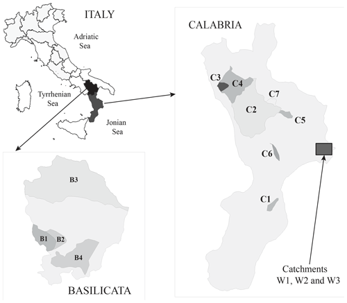
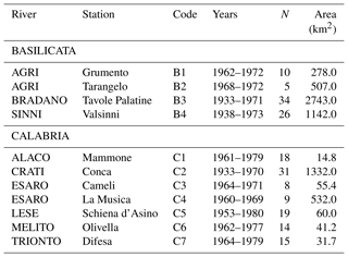
The Italian Hydrographic Service (SIMI) has published long-term measurements of daily and monthly suspended sediment load (SSL) on many catchments throughout the country. In the present contribution, monthly measurements of SSL, which were collected on 11 rivers located in Calabria, and Basilicata, have been used for analysis. This step required also a preliminary aggregation of the data to generate the annual datasets of sediment yield (see Table 1 and Fig. 2 for details).

These datasets have been integrated by 3 long-term records of sediment yield obtained in three experimental catchments (W1, W2, and W3) located in Calabria (see Porto et al., 2004). In this case, the original measurements, collected at event scale, have been aggregated at annual scale to make them comparable with the previous datasets.

Figure 2 Location of the catchments investigated in this study.

More specifically, the 11 datasets were used to derive the growth curve (Eq. 3) for the entire region, here assumed as a unique homogeneous area, while the three catchments W1, W2, and W3 were used to test the validity of the Eq. (3) on independent datasets located in the same region.

In other words, the hierarchical approach proposed in this study consists of two levels: (1) the first level aimed at calculating the 3 parameters (Λ_∗, Θ_∗ and λ₁) of the Eq. (3) on the area where the catchments are located. In this respect, a comparison between the empirical and theoretical CDFs of γ was performed; (2) the second level served to validate the Eq. (3) on the three independent datasets for which the empirical CDFs of the variable x are available.

Table 1 Details of stream gauges and rivers considered in this study.

3 Results and discussions

3.1 Model calibration

The analysis carried out at the first level required the basic assumption that the entire region can be considered homogeneous with respect to the skewness coefficient, γ and the coefficient of variation, CV (see Fiorentino et al., 1987; Beran et al., 1986). However, considering the short length of some historical datasets (N<10 years), some preliminary adjustments of these records were necessary. More specifically, based on geomorphic similitude, the two datasets of River Agri (see Table 1) were bulked into one single dataset with N=15; the same assumption was made for the two records of River Esaro for which a final single dataset with N=17 was obtained.

As explained above, in the first step of this analysis, the TCEV model required the estimation of the regional parameters Λ_∗ and Θ_∗ referred to these new nine series. This analysis was conducted using the procedure suggested by Fiorentino and Gabriele (1985) that led to the following ML estimates of the two parameters:

$$\begin{array}{}\text{(6)}& {\mathrm{\Lambda }}_{\ast }=\mathrm{0.675};{\mathrm{\Theta }}_{\ast }=\mathrm{11.574}\end{array}$$

In order to verify the homogeneity of the entire region with regard to γ, Monte Carlo experiments were performed for generating theoretical sequences having a fixed size N and distributed according to a TCEV model with regional parameters given by Eq. (6).

The CDF of the empirical skewness related to the 9 samples and that generated by the regional model are compared in Fig. 3. The theoretical CDF was obtained using a Monte Carlo technique based on 20 000 synthetic series having a sample size N equal to the mean value calculated from the empirical datasets.

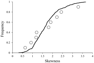
Figure 3 Comparison between the empirical CDF of the skewness coefficient calculated from the nine datasets and the regional CDF obtained from the theoretical distribution.

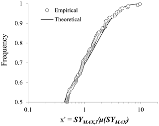
Figure 4 Comparison between empirical and theoretical CDF of the variable x^′ for the 9 investigated datasets.

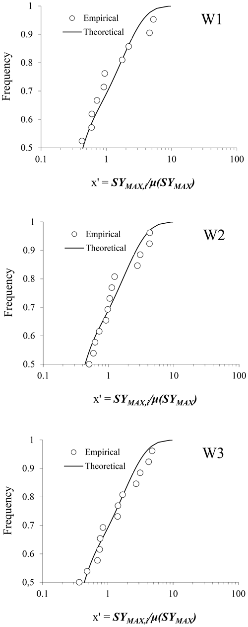
Figure 5 Comparison between empirical and theoretical CDFs of the variable x^′ for the 3 independent datasets (W1, W2 and W3).

Even if a perfect overlapping cannot be expected considering the limited number of datasets, Fig. 3 shows a certain ability of the TCEV distribution to reproduce the empirical skewness CDF.

The second step of the analysis is based on the assumption that the investigated region should be divided into smaller homogeneous areas, named sub-regions, in which the λ₁ parameter can be assumed constant. Because the λ₁ parameter is related to CV by the following equation:

$$\begin{array}{}\text{(7)}& \text{CV}={\displaystyle \frac{\mathrm{0.577}}{\log {\mathrm{\Lambda }}_{\mathrm{1}}+\mathrm{0.251}}}\end{array}$$

this is equivalent to defining sub-regions within which the coefficient of variation of the individual series can be assumed constant. Unfortunately, the number of series available in the entire region (9 datasets) is not enough to proceed with a further geographic subdivision and this hypothesis could not be considered. In the light of this limitation, the analysis was carried out considering a unique homogeneous region even at the second hierarchical level. Consequently, according to Arnell and Gabriele (1988), the value of Λ₁ was determined using the TCEV distribution with the regional values of Λ_∗ and Θ_∗ given by Eq. (6). Using the data obtained from the historical datasets, the parameters Λ₁ and α assume the following values:

$$\begin{array}{}\text{(8)}& {\mathrm{\Lambda }}_{\mathrm{1}}=\mathrm{5.974};\mathit{\alpha }=\mathrm{8.776}\end{array}$$

Figure 4 shows that the growth curve calculated by the Eq. (3), with the parameters given by the Eqs. (6) and (8) fits very well the higher values ($f\left(x^{\prime }\right)>\mathrm{0.5}$) of the x^′ empirical distribution suggesting that the hypothesis of unique homogeneous region is plausible.

3.2 Model performance

The regional growth curve given by the Eq. (3) with the calibrated values of the 4 parameters (Λ_∗, Θ_∗ , λ₁ and α) was tested on three independent datasets available for three experimental catchments (W1, W2, and W3) located in Calabria (see Fig. 2). Details of these catchments are reported elsewhere (see Ferro and Porto, 2000). Here, only the CDFs of the empirical variable x^′ are considered and the comparison with the theoretical distribution is reported for each catchment in Fig. 5.

The visual inspection of the three graphs in Fig. 5 suggests that, the model fits reasonably well the higher values ($f\left(x^{\prime }\right)>\mathrm{0.5}$) of the x^′ empirical distributions suggesting that the regional growth curve is very robust and can be used for obtaining reliable predictions even for large events.

4 Conclusions

Prediction of sediment yield generated by large events is very important in areas not covered by monitoring stations or for the areas with limited observational periods. Based on a previous contribution by Porto and Callegari (2019), the study presented herein reports a regional investigation carried out in Southern Italy aimed at evaluating the frequency distribution of sediment yield. The procedure applied in this contribution is based on the use of the TCEV model and its hierarchical approach to get reliable estimates of the regional parameters of the distribution. The choice is due to the ability of the TCEV distribution to reproduce the skewed empirical distributions of sediment yield observed in many historical datasets and to generate estimates of sediment yield associated with a fixed return time. Overall, the study demonstrated that even if the TCEV distribution was conceived to provide estimates of peak flow, its basic assumptions and its hierarchical procedure can be used to predict sediment yield at regional scale.