Influence of cylindrical obstacle concentration on flow dynamics in channels: a computational approach to optimizing geometric configurations

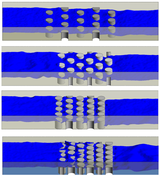
This study investigates the impact of cylindrical obstacle concentration (C) on flow dynamics in low-slope channels using ANSYS Fluent. Cylinders (D = 12 cm, L = 15 cm) were arranged with varying axial and lateral spacings, producing concentrations from 9 % to 64 %. Simulations under critical flow conditions with a 1 m s⁻¹ inlet velocity employed the VOF method and Kw turbulence model to assess velocity, turbulence, pressure, and shear stress. Results show that increased obstacle concentration enhances energy dissipation, with turbulence intensity decreasing from 0.08 to 0.03–0.05 m² s⁻². Wall shear stress rises to 6.5 Pa at 64 % C due to flow constriction, while velocity deficits downstream reduce from 40 %–50 % to 20 %–30 %. These findings underline how obstacle arrangement influences flow resistance and energy loss. It also provide quantitative design insights for improving hydraulic performance in low-slope floodplain environments. These results directly inform flood resilience strategies and infrastructure design by illustrating how controlled obstacle density can enhance energy dissipation and manage flow resistance.

1 Introduction

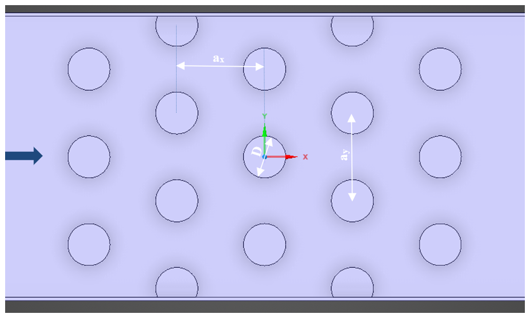
Channel flow around obstacles (e.g., bridge piers, vegetation) critically affects sediment transport, energy dissipation (Gharbi et al., 2016; Nasim et al., 2019), flood management, and infrastructure design (Mahjoub et al., 2024a; Schlömer and Herget, 2023). Significant modeling gaps persist regarding how cylindrical obstacles modify flow behavior in low-gradient floodplains. This study addresses this central research question to clarify how finding can inform resilient infrastructure design in flat terrains (Schlömer and Herget, 2023; Mahjoub et al., 2024b). Using CFD (Fluent) to solve Navier-Stokes equations (Tran, 2015; Rasha et al., 2023; Tafarojnoruz and Lauria, 2020), we analyze cylindrical obstacle concentration ($C=f(D,a_x,a_y)$) impacts on velocity, turbulence, and pressure. Figure 1 shows a configuration.

This work bridges theory and practice to enhance urban/rural water management. Key questions:

• How do cylindrical obstacles alter low-slope floodplain flows?

• How does obstacle concentration (C) affect velocity, turbulence, and pressure?

• How can findings improve flood resilience and infrastructure design?

Subsequent sections present methodology, key results, and theoretical/practical implications for flow systems.

2 Methodology

This methodology quantifies obstacle concentration effects via VOF/SIMPLE-solved equations and multi-concentration simulations capturing fluid-structure interactions.

2.1 Basic Definitions used in this analysis

This analysis examines key parameters in obstacle-flow interactions underpinning the numerical model.

2.1.1 Obstacle Concentration

Concentration C is defined by the spatial arrangement of obstacles regularly spaced in both longitudinal a_x and transverse a_y directions. These parameters (a_x, a_y) were selected to systematically span a range of obstacle densities (9 % to 64 %) to simulate varying degrees of hydraulic resistance encountered in natural floodplains. The concentration is given by:

$$\begin{array}{}\text{(1)}& C={\displaystyle \frac{D^{\mathrm{2}}}{\left(a_x\cdot a_y\right)}}\end{array}$$

This concentration C represents the obstacles density within the flow and plays a crucial role in determining these obstacles impact on the flow dynamics.

2.1.2 Reynolds Decomposition

Reynolds decomposition separates flow into mean and fluctuating components (Aksel, 2023). The Reynolds decomposition of the velocity field u is expressed as:

$$\begin{array}{}\text{(2)}& u=\stackrel{\mathrm{‾}}{u}+u^{\prime }\end{array}$$

Reynolds decomposition separates mean $\stackrel{\mathrm{‾}}{u}$ and turbulent u^′ components, enabling RANS derivation.

2.1.3 Reynolds number

The global Reynolds number for this study, defined as:

$$\begin{array}{}\text{(3)}& Re={\displaystyle \frac{U{R}_{\mathrm{H}}}{\mathit{\upsilon }}}\end{array}$$

Where U is the bulk velocity and R_H is the Hydraulic radius, and υ is water viscosity. This dimensionless parameter serves as a standardized indicator of the inertial dominance within the channel, ensuring the study remains consistent with high-energy floodplain dynamics.

2.1.4 Turbulent Kinetic Energy

Turbulent kinetic energy (TKE) represents the energy contained in the flow of turbulent fluctuations (Kosari et al., 2018). It is calculated as the sum of the velocity fluctuations variances:

$$\begin{array}{}\text{(4)}& {\mathit{\kappa }}_T={\displaystyle \frac{\mathrm{1}}{\mathrm{2}}}(\stackrel{\mathrm{‾}}{{u^{\prime }}^{\mathrm{2}}}+\stackrel{\mathrm{‾}}{{v^{\prime }}^{\mathrm{2}}}+\stackrel{\mathrm{‾}}{{w^{\prime }}^{\mathrm{2}}})\end{array}$$

Where $u^{\prime },v^{\prime }$ and w^′ are the fluctuating velocity components, and $\stackrel{\mathrm{‾}}{{u^{\prime }}^{\mathrm{2}}}$,$\stackrel{\mathrm{‾}}{{v^{\prime }}^{\mathrm{2}}}$ and $\stackrel{\mathrm{‾}}{{w^{\prime }}^{\mathrm{2}}}$ represent the time-averaged variances of these fluctuations.

2.1.5 Water surface tension

Water surface tension arises from cohesive forces between surface molecules. For simulations, the value of 0.072 N m⁻¹ (25 °C) is adopted. It is modeled via the Continuum Surface Force approach.

$$\begin{array}{}\text{(5)}& F_{\mathrm{CSF}}=\mathit{\sigma }\mathit{\kappa }\mathit{\delta }\left(r\right)n\end{array}$$

The surface tension coefficient σ is a fluid property, while κ represents interface curvature. The Dirac delta function δ localizes the tension force at the interface.

2.1.6 Wall Shear Stress

Wall shear stress τ_w, critical for near-boundary flow analysis, quantifies frictional forces at fluid-solid interfaces. Computed from near-wall velocity gradients in ANSYS Fluent, it follows:

$$\begin{array}{}\text{(6)}& {\mathit{\tau }}_{\mathrm{w}}=\mathit{\mu }\cdot {\left.{\displaystyle \frac{\partial u}{\partial z}}\right|}_{z=\mathrm{0}}\end{array}$$

where μ is the fluid dynamic viscosity and $\partial u/\partial z$ represents the velocity gradient normal to the wall. Accurate wall shear stress governs sediment transport, erosion, and hydraulic structure stability predictions.

2.1.7 Strouhal number

The Strouhal number (S_t) is a dimensionless parameter that characterizes the oscillatory behavior of fluid flow (Jiang and Cheng, 2017; Blevins, 1977; Williamson and Govardhan, 2004), particularly in vortex shedding phenomena. It is defined as:

$$\begin{array}{}\text{(7)}& S_t={\displaystyle \frac{fD}{U}}\end{array}$$

where f= vortex shedding frequency, D = characteristic length (cylinder diameter/obstacle width), U = free-stream velocity.

This framework analyzes cylindrical obstacle dynamics via: Reynolds decomposition (turbulence), TKE (intensity quantification), and biphasic flow (air-water interactions) and forms the foundation of the numerical methodology.

Figure 1 Schematic diagram of one of the Obstacle configurations in this study (Top View).

2.2 Description of the Hydrodynamic simulation

2.2.1 Governing equations

The study employs the incompressible RANS equations solved via the VOF method. While Large Eddy Simulation (LES) is recognized for resolving instantaneous sub-grid scales, the RANS framework was strategically selected here as the optimal tool for interpreting macroscopic hydraulic variables (Mahjoub et al., 2024b; Kosari et al., 2018; Roulund et al., 2005; Senturk et al., 2023), specifically bulk energy dissipation and mean resistance coefficients. Given that the engineering objective is to quantify global flow behavior rather than transient fine-scale fluctuations, the RANS approach provides a degree of fidelity that is precisely calibrated to the scale of the outputs required, ensuring a robust balance between computational efficiency and the precision needed for floodplain modeling, consistent with prior hydraulic applications (Aksel, 2023; Roulund et al., 2005b; Senturk et al., 2023).

Mass continuity

The mass continuity equation ensures the conservation of mass and it is expressed as:

$$\begin{array}{}\text{(8)}& {\displaystyle \frac{\partial \mathit{\rho }}{\partial t}}+\mathrm{\nabla }\cdot \left(\mathit{\rho }\mathit{u}\right)=\mathrm{0}\end{array}$$

where ρ is the fluid density, and u is the mean velocity vector.

Momentum conservation equation

The momentum conservation equation describes the balance of forces acting on a fluid and it is expressed as follows:

$$\begin{array}{}\text{(9)}& \mathit{\rho }\left({\displaystyle \frac{\partial \mathit{u}}{\partial t}}+\mathit{u}\cdot \mathrm{\nabla }\mathit{u}\right)=-\mathrm{\nabla }p+\mathrm{\nabla }\cdot \left[\mathit{\mu }\right(\mathrm{\nabla }u+\mathrm{\nabla }{u}^T\left)\right]+f_{\mathrm{s}}+f_{\mathrm{g}}\end{array}$$

Fluid density is denoted by ρ, velocity vector by u, and time by t. Pressure is p, dynamic viscosity μ characterizes shear resistance, f_s accounts for interfacial surface tension, and f_g represents gravitational acceleration. This framework comprehensively models fluid motion.

2.2.2 Biphasic Flow, Volume Fraction Equation

Biphasic flow involves coexisting distinct phases (Kosari et al., 2018). The Volume of Fluid (VOF) method (Hirt and Nichols, 1981) tracks interfaces using volume fraction α per computational cell. The equation governing biphasic flow in the VOF method is:

$$\begin{array}{}\text{(10)}& {\displaystyle \frac{\partial \mathit{\alpha }}{\partial t}}+\mathit{u}\cdot \mathrm{\nabla }\mathit{\alpha }=\mathrm{0}\end{array}$$

The dimensionless parameter α ($\mathrm{0}\le \mathit{\alpha }\le \mathrm{1}$) indicates phase distribution. Mass conservation for the tracked phase is maintained by solving the volume fraction equation alongside the Navier-Stokes equations.

2.2.3 Turbulence closure

The TKE transport equation governs convection-diffusion, shear/buoyancy production, and viscous dissipation (Schiestel, 2006). Turbulence closure challenges in hydraulic engineering demand rigorous calibration and validation for reliable approximations.

2.3 Simulation specifications

2.3.1 Initial and boundary conditions

This laboratory-scale model employs a 10 m × 0.8 m × 0.6 m canal. Initial conditions (0.1 m depth, 1 m s⁻¹ velocity) ensure dynamic similarity (Mahjoub et al., 2024a; Chanson, 2006). To provide essential context for the turbulence modeling, the global Reynolds number of the flow was calculated as Re=10⁵ confirming a fully turbulent regime consistent with standard floodplain dynamics. Furthermore, the Froude number was determined to be Fr=1.01 indicating that the simulations were conducted under critical flow conditions, which is a key threshold for assessing energy dissipation and wave stability in open channels. The VOF method models air-water flow with no-slip walls. Pressure-velocity coupling applies first-order upwind (dissipation/stability) and second-order upwind (momentum/TKE/accuracy) schemes, with global time stepping for convergence.

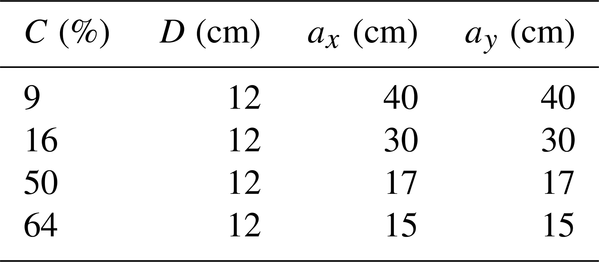
Table 1 Configuration Parameters for Different Obstacle Concentrations.

2.3.2 Mesh configuration

All configurations used 2 cm elements, 0.4 max skewness, enhanced smoothing. Curvature: 0.02 cm min, 10° angle. Inflation: 0.272 ratio, 5 layers, 1.2 growth. Mesh independence confirmed. Figure 2 shows mesh refinement near obstacles (50 % concentration), capturing complex phenomena for accurate local interaction simulation.

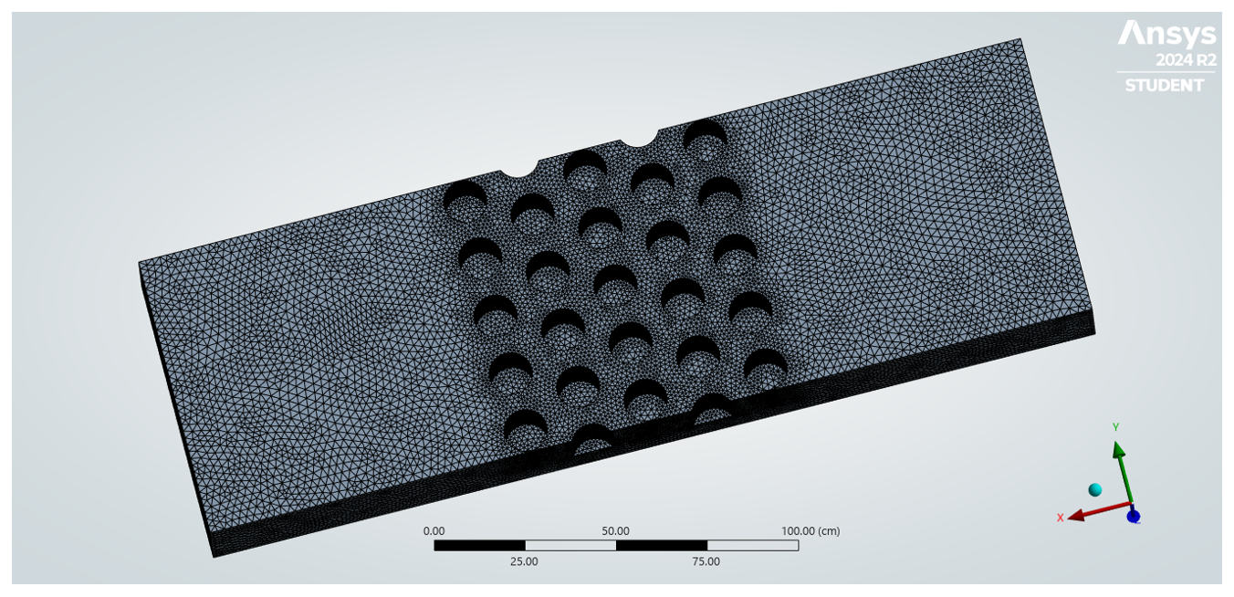
Figure 2 Example of the fluid domain sketch of the study after meshing, in the case of a 50 % concentration.

2.3.3 Validation/Calibration of the Numerical Model

Three closure models were validated: k−ε, K−ω and SST. All demonstrated comparable accuracy near obstacles. However, based on literature demonstrating the K−ω model's efficacy in flows with adverse pressure gradients and separation (Aksel, 2023; Roulund et al., 2005; Senturk et al., 2023; Cassan and Laurens, 2016), it was selected to ensure reliable fluid behavior representation.

3 Results

This study quantifies cylindrical obstacle concentration effects on channel hydrodynamics. Analysis resolves flow kinematics (velocity, turbulence, wakes) to interpret forces/pressure, revealing concentration-dependent resistance, dissipation, and shear stress for hydraulic design.

3.1 Flow Kinematics – Time-Averaged Analysis

The validation framework compares experimental data from Tran (2015) with numerical outputs across concentrations, as shown in Fig. 3. It shows the physical fish pass (left) with tilted flows and its numerical model (right) with lateral flow contractions in red, transcritical transition in yellow and, resting zone in blue.

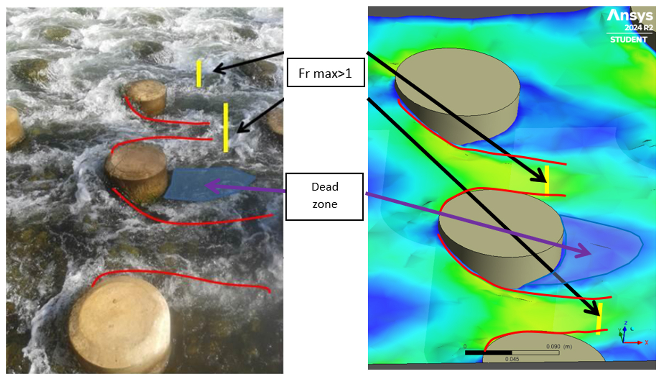
Figure 3 Comparison between a photograph of flow in an actual fish pass and numerical model results for the same obstacle geometry.

3.2 Velocity Field and Streamline Patterns

Figure 4 shows spatial variations of time-averaged wake velocity magnitude across obstacle concentrations, consistent with Tran (2015) and Bretón et al. (2013). Concentration critically influences flow behavior through velocity reduction, shear layers, wake recovery, and dissipation. Lower concentrations (9 %, 16 %) yield minimal upstream perturbation and moderate wake velocity reduction. Higher concentrations (50 %, 64 %) generate significant immediate velocity deficits downstream due to intensified wake interactions and vortex formation. At 64 % concentration, wake velocity drops below 25 % of free-stream, indicating substantial dissipation and aligning with decreasing $U_{\mathrm{wake}}/U_{\mathrm{\infty }}$ trends.

Figure 4 Velocity Magnitude Contours for Different Obstacle Configurations.

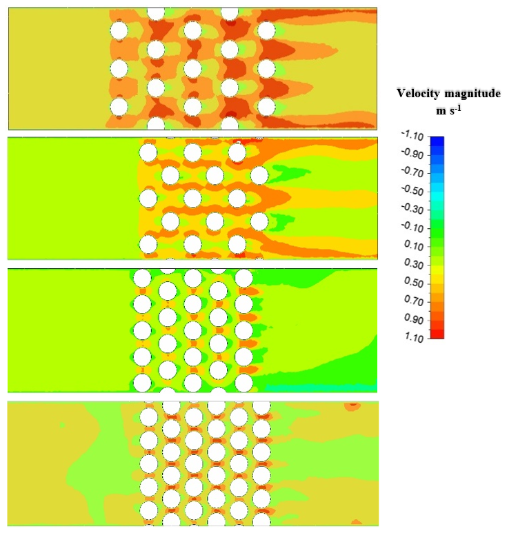
Figure 5 presents vertical velocity distributions across obstacle concentrations, confirming reduced velocities with increasing density, particularly pronounced at lower $Z/h$. Profiles grow increasingly asymmetric with concentration, exhibiting steeper velocity gradients and enhanced momentum loss in the near-wake region, aligning with Fig. 4 patterns.

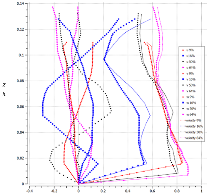
Figure 5 Velocity Profiles at Different Obstacle Concentrations (Vertical distribution of velocity components for varying obstacle concentrations.

3.3 Turbulence Intensity and Vortex Formation

Obstacle concentration critically governs turbulence and vortex dynamics. Low concentrations (9 %–16 %) yield periodic shedding (S_t≈0.2–0.25), TKE ∼ 0.08 m² s⁻², and 40 %–50 % deficits. High concentrations (50 %–64 %) induce chaotic flows: disrupted shedding (S_t≈0.1–0.15), TKE dissipation (0.03–0.05 m² s⁻²), and reduced deficits (20 %–30 %) from momentum redistribution. This aligns with turbulence cascade theory (Nikora and Roy, 2012), where obstructions fragment eddies, accelerating dissipation and informing hydraulic design for erosion control and water retention.

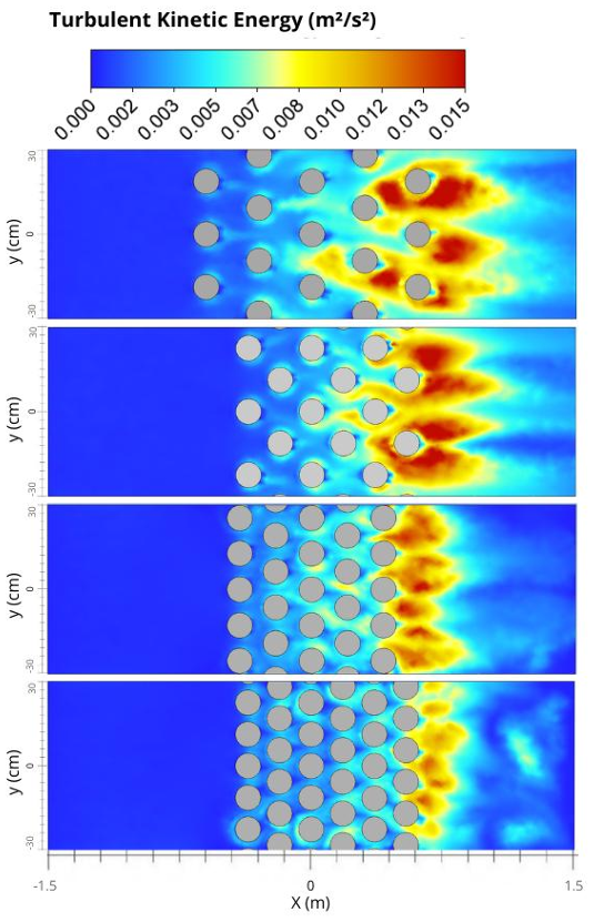
Figure 6 Distribution of Turbulent Kinetic Energy (TKE) downstream of obstacles for varying configurations.

3.4 Wall Shear Stress Distribution

Wall shear stress escalates with obstacle concentration (Fig. 7). Low densities (9 %–16 %) yield uniform stress < 2.0 Pa (blue zones). Medium (25 %–36 %) induces localized peaks (3.0–5.0 Pa; yellow zones) from constriction. High densities (50 %–64 %) exhibit > 6.5 Pa (orange zones) due to turbulent wake interactions and Navier-Stokes pressure effects. This signifies:

• Increased flow resistance/erosion risks

• Sediment hotspots requiring scour protection

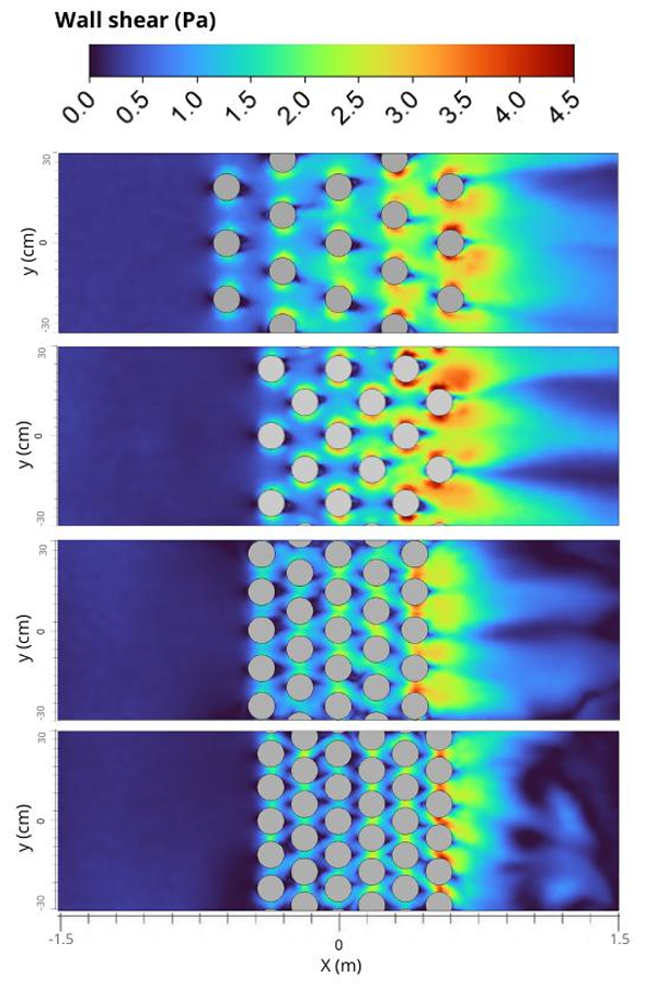
Figure 7 Wall Shear Stress Distribution for Different Obstacle Configurations – Numerical Simulation Results.

3.5 Effect of Obstacle Concentration on Water Surface Profiles

Figure 8 shows water surface profiles (x-z plane at y=0) for obstacle concentrations (9 % red, 16 % blue, 50 % black, 64 % pink) under critical flow (inertial/gravitational balance). Three distinct regions exhibit unique behaviors: upstream ($x<-\mathrm{0.5}$ m), obstacle zone (−0.5 m $<x<\mathrm{0.5}$ m), and downstream (x>0.5 m), necessitating regional analysis.

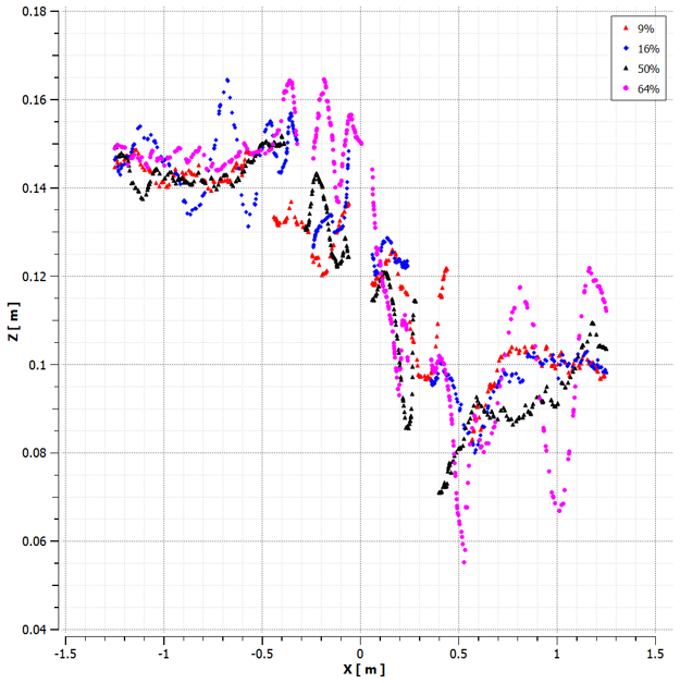
Figure 8 Water Surface Profile in the (x, z) Plane at y = 0 for Different Obstacle Concentrations.

Upstream, flow is uniform with minimal surface elevation changes, though higher concentrations (50 %, 64 %) show slight rises due to early blocking effects.

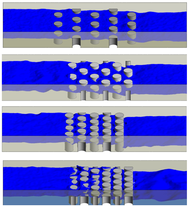
Within the obstacle zone, concentration dictates disturbance: low densities (9 %, 16 %) cause minor deviations, while high densities (50 %, 64 %) produce significant peaks/troughs (±20 mm) and potential recirculation (Fig. 9), indicating strong resistance and energy loss.

Downstream, recovery length increases sharply with concentration: flow stabilizes quickly after sparse arrays (9 %: 1.2 m; 16 %: 1.8 m) but requires > 2.5 m for dense arrays (50 %, 64 %) due to persistent eddies. Higher concentrations extend recovery by intensifying blocking effects and energy dissipation, aligning with established obstacle flow dynamics (Britter and Hanna, 2003; Tran, 2015).

Figure 9 Water Surface Profiles for Different Obstacle Concentrations.

4 Discussion and conclusion

4.1 Discussions

Obstacle concentration critically controls water surface deformation and turbulence intensity. Low densities (9 %, 16 %) cause mild surface fluctuations (±3 mm), while high densities (50 %, 64 %) induce localized elevations up to 20 mm due to clustering and enhanced drag. Turbulence intensity increases by nearly 40 % in high-density wakes. Recovery length extends significantly with concentration, from 1.2 m for sparse arrays to over 2.5 m for dense ones, due to persistent wake interactions, aligning with prior studies (e.g., Nepf, 2012; Tanino and Nepf, 2008). Hydraulic resistance (Darcy-Weisbach friction factor) rises substantially, 15 % for low concentrations and over 40 % for high densities, reducing conveyance capacity. This is vital for flood management, where obstacles can regulate flows and dissipate energy.

4.2 Conclusions

Obstacle concentration critically controls water surface deformation and turbulence. Low densities (9 %, 16 %) cause mild surface fluctuations (±3 mm), while high densities (50 %, 64 %) induce localized elevations up to 20 mm due to clustering. Recovery length increases significantly with concentration, extending from 1.2 m for sparse arrays to over 2.5 m for dense ones because of persistent wake interactions. Hydraulic resistance coefficients rise 15 %–40 % with higher densities, reducing conveyance capacity, which is vital for flood and sediment management. These results provide a foundation for designing hydraulic structures and optimizing flow management. Future work should include experimental validation, 3D analysis, and exploring obstacle shape and arrangement.