Investigation of Uncertainties in Multi-variable Bias Adjustment in Multi-model Ensemble

Post-processing methods such as univariate bias adjustment have been widely used to reduce the bias in the individual variable. These methods are applied to variables independently without considering the inter-variable dependence. However, in compound events, multiple atmospheric factors occur simultaneously or in succession, leading to more severe and complex impacts. Therefore, a multi-variable bias adjustment is necessary to retain the inter-variable dependence between the atmospheric drivers. The present study focuses on a multi-variable bias adjustment of surface air temperature and relative humidity in a multi-model ensemble. We investigated added values and biases before and after adjusting the variables. There are gains and losses throughout the process of adjustment. The bias adjustment effectively reduces bias in surface air temperature; however, it shows bias amplification for relative humidity at higher altitudes. Added values were improved at lower altitudes but showed reductions in surface air temperature at higher altitudes. Overall, the bias adjustment shows improvement in reducing bias over low-altitude urban areas, encouraging its application to assess compound events. These findings highlight a potential bias adjustment approach for the regions with a constraint on observational data.

1 Introduction

Quantifying the impact of climate change at a regional scale requires reliable, unbiased information. General circulation models (GCMs) have been our main source of knowledge on the past and future climate; however, regional-scale surface and atmospheric drivers of climate extremes are not well resolved in GCMs (Ayar et al., 2015). Therefore, regional climate models (RCMs) are widely used to dynamically downscale the GCMs. RCM products have been known to provide a clearer understanding of surface-induced processes compared to the parent model. However, they still have uncertainties, contributing to biased model output (Giorgi, 2019). Some of these uncertainties are related to the structural differences and internal variability in climate models, while some are related to the boundary conditions and bias propagation from GCM to RCM (Addor et al., 2016).

Bias Adjustment

Bias adjustment methods are the primary post-processing tools to reduce model bias. Many methods have been developed and applied to post-process climate simulations. Most bias adjustment methods reduce the bias by adjusting the statistical features, such as quantiles (Themeßl et al., 2012) and variance (Berg et al., 2012). Some methods focus on adjusting the boundary conditions of GCM to improve the RCM simulations (Bruyère et al., 2013; Kim et al., 2023). However, these methods are applied to single variables (univariate) at a time, i.e., independently (Hempel et al., 2013). Due to this limitation, the inter-variable dependence is often not considered, which might lead to misinterpretation of the results. Past research suggests that the single-variable bias adjustment methods suffice the specific regional impact studies (Casanueva et al., 2018). However, inter-variable dependence is significant for assessing compound events where multiple variables play a crucial role (Zscheischler and Seneviratne, 2017). Multi-Variable Bias Adjustment (MBA) methods were, thus, developed for consistent impact assessment. However, similar to univariate bias adjustments, MBAs focus on correcting the statistical features and lack consideration of physical parameters such as underlying terrain. Topography is essential when the multiple surface-sensitive drivers regulate compound events or for understanding the hydrological processes over complex terrain. Some studies incorporated topography to downscaling reanalysis products and climate models (Gupta and Tarboton, 2016; Fiddes et al., 2022) and noted a relative advantage of acquiring reliable climate information over complex terrain. However, our study considers topography exclusively for bias adjustment purposes, focusing on the drivers of heat stress, the surface air temperature, and relative humidity (Davis et al., 2016), which are sensitive to the underlying terrain.

This study investigates the uncertainties associated with the bias adjustment method, based on topographical adjustment of surface air temperature and relative humidity in a multi-model ensemble of GCM-RCM. Therefore, this study refers “multi-variable” to model simulated surface air temperature and specific humidity (which has been used to estimate relative humidity).

2 Data and Method

We analyzed the 2 m surface air temperature (T2) and estimated relative humidity (RH) from an ensemble of Global- (GCM) and Regional-Climate Model (RCM) simulations performed by Nayak et al. (2018) over Japanese land. The ensemble includes three RCMs, NHRCM, -NRAMS, and WRF, forced by Japanese 25-year Reanalysis (JRA25) and three GCMs, CCSM4, MIROC5, and MRI-CGCM3. The RCM simulations are at 20 km horizontal grid spacing for the present climate (1981–2000) and future climate (2081–2100) under RCP4.5. The analysis in this study is based only on the present climate. For validation, the daily observation data on T2 (1981–2000), RH (2008–2020), and Elevation (DEM) are obtained from the NARO gridded (1 km grid spacing) dataset (Ohno et al., 2016). Hourly simulated climate data was aggregated to their daily means and were regridded on a reference Lat–Long grid with 20 km spacing with the inverse distance weighting method for a consistent comparison (Dodson and Marks, 1997).

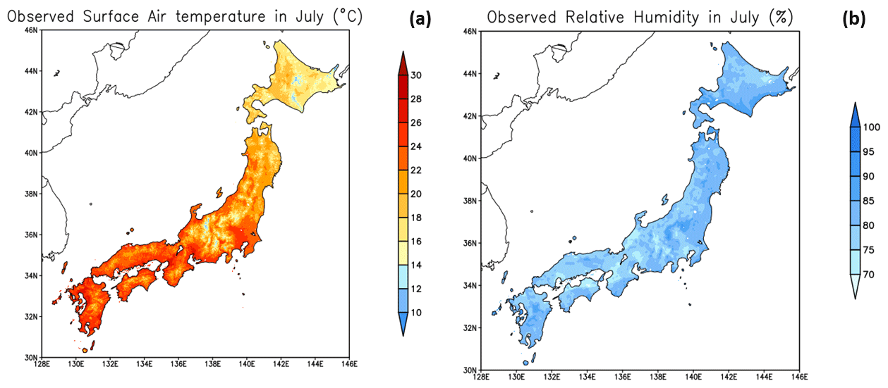
Figure 1 (a) Observed mean surface air temperature, T2 (°C), in July for the period 1981–2000; Observed mean relative humidity, RH (%), in July for the period 2008–2020.

The Multi-variable Bias Adjustment is based on the topographical adjustment of surface climate variables. We follow the Micromet framework detailed in Liston and Elder (2006). This method was initially developed to adjust individual variables from the weather station dataset; however, we adapted it to adjust multiple climate variables.

Ensemble simulations obtained from the study of Nayak et al. (2018) provide specific humidity instead of RH. Therefore, we obtain RH through the empirical method.

Figure 2 Process of RH estimations and adjustment to topography.

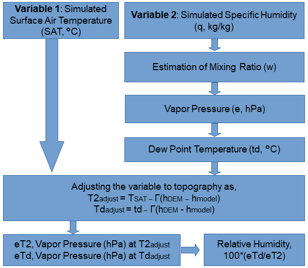
First, we calculate the mixing ratio and vapor pressure (hPa) from model simulated specific humidity and surface pressure (Wallace and Hobbs, 2006), which are used to calculate the dew point temperature as detailed in Liston and Elder (2006). The adjustment factor, h, is estimated using the lapse rate, Γ (°C km⁻¹), NARO elevation, h_DEM (in km), and model elevation data h_model (in km),

$$\begin{array}{}\text{(1)}& h=\mathrm{\Gamma }(h_{\mathrm{DEM}}-h_{\mathrm{model}})\end{array}$$

Once we obtain the adjustment factor, T2 and dew point temperature are adjusted and used for the RH estimations according to the Micromet framework. The Bias adjustment is applied to each of the GCMs, RCMs, and JRA25. Ensemble means of the GCMs, GCM-forced RCMs, and JRA25-forced RCMs are estimated before and after the adjustment. Here, we primarily focus on the ensemble means, but more information on biases in each model is shown in the Supplement.

We also assess the added value (AV) of the RCMs to examine the impact of bias adjustment. The added value (AV) issue has been central to the climate model community (Rummukainen, 2015). AV is found to depend on model grid resolutions (Lenz et al., 2017), physical processes such as convective processes (Schaaf and Feser, 2018); as well as complex topography regions like mountainous terrains (Torma et al., 2015), which indicates the AV of the downscaled product is most likely when local and regional scale processes are essential for the climate and characteristics of the region. We use a metric of squared errors in climate variable (X) (Di Luca et al., 2013).

$$\begin{array}{}\text{(2)}& \mathrm{AV}={\left(X_{\mathrm{GCM}}-X_{\mathrm{Observation}}\right)}^{\mathrm{2}}-{\left(X_{\mathrm{RCM}}-X_{\mathrm{Observation}}\right)}^{\mathrm{2}}\end{array}$$

The added value defined here retains the units of the climate variables in the metric. It is positive whenever the biases in the RCMs are smaller than in the GCMs.

Before moving forward to the next section, we would like to note that this methodology adjusts the drivers to the underlying topography. Thus, it is irrelevant to the long-term trend and data training period.

3 Results and Discussion

Here, for brevity, we show the results for July, one of the hottest months in Japan. Figure 3 shows the mean bias in surface air temperature during July before (a, c) and after (b, d) applying the adjustment factor to the RCM ensemble – forced by three GCMs – MRI-CGCM3, CCSM4, and MIROC5 (Fig. 3a, b) and JRA25 reanalyses (Fig. 3c, d). Mean bias is a 20-year mean of difference between daily model and observational data.

Here, we examined the model ensemble mean only and observed negative bias over most of the Japanese land and weak positive bias over northern parts for the GCM forced RCM ensemble (Fig. 3a). On the other hand, the JRA25 forced RCM ensemble shows weak bias (Fig. 3c). Differences in bias before and after adjustment for each model are shown in Supplement Figs. S1–S6.

After applying the adjustment factor, the bias has prominently reduced, as seen in the rightmost panels of Fig. 3, which shows the difference in the absolute value of bias before and after adjustment.

The positive value indicates that the magnitude of bias before the adjustment was larger than after the adjustment, indicating bias reductions.

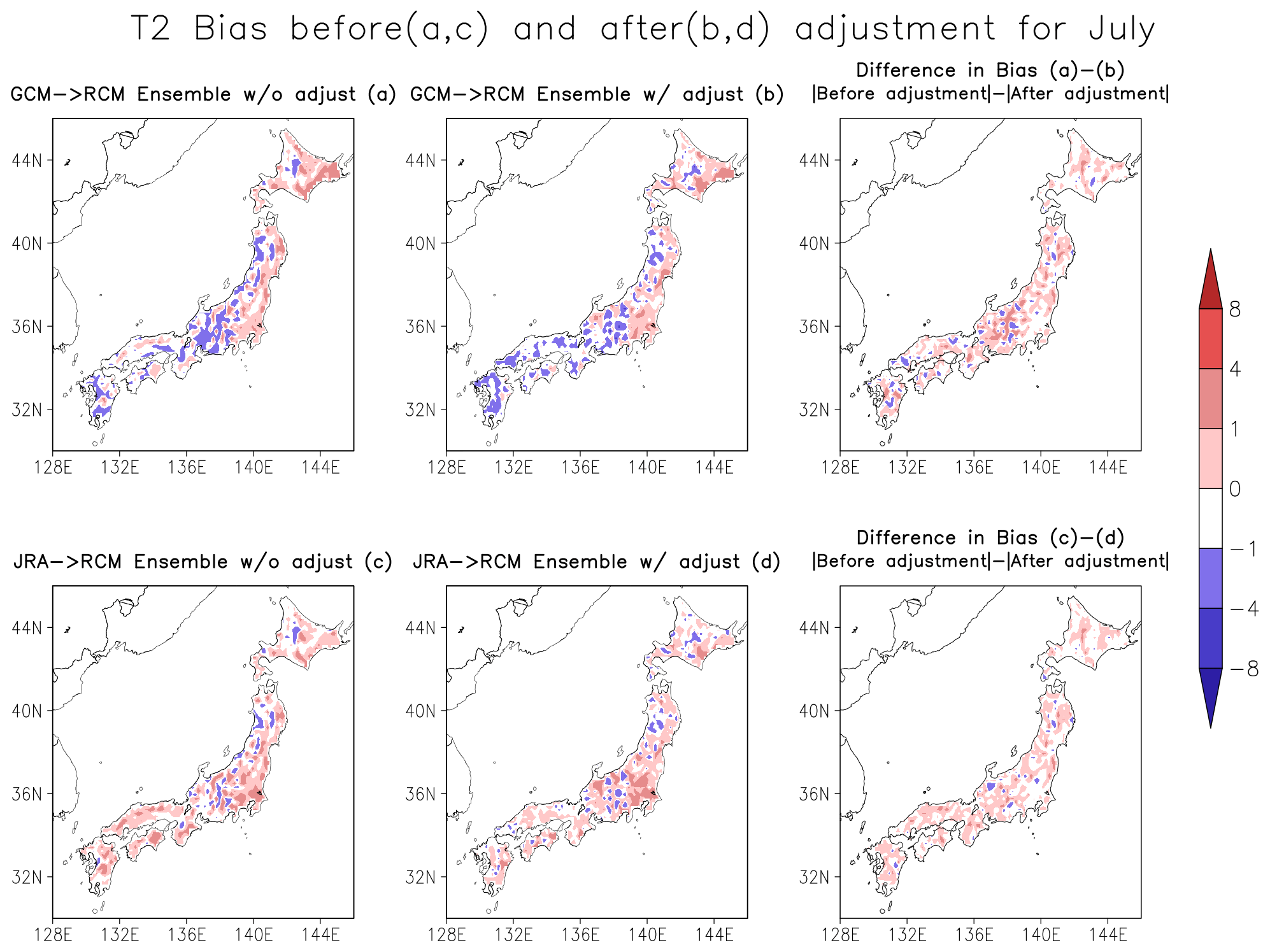
Figure 3 T2 bias (°C) before (a, c) and after applying adjustment factor (b, d) to GCM- (a, b) and JRA25-forced RCM ensemble simulations (c, d).

We indicate bias reductions from the perspective of absolute values as these biases are both positive and negative and would have obscured examining bias reductions otherwise.

As discussed earlier, the dependence structure between the climate variables is crucial for consistent assessment of compound events such as heat stress. The multi-variable bias adjustment includes the adjusted T2 while estimating the RH to consider the inter-variable relationship between T2 and RH. Here, the inter-variable dependence is considered through the empirical relationship between T2 and RH and not through the statistical features such as quantiles or probability distributions. In Fig. 4, we compare relative humidity during July before (b) and after (a), applying the adjustment factor to the RCM ensemble. We show the comparison for GCM forced ensemble because humidity data is available for GCM forced ensemble only.

Intriguingly, after applying the adjustment factor (Fig. 4b), coastal regions and the Kanto plain of central Japan show a reduction in bias, yet mountainous areas of northern and central Japan display added bias. On the other hand, in the case of T2, we observe cold bias at high altitudes (Table 1). These results indicate that the impacting factors could originate from the empirical formulation of bias adjustment and calculation of RH.

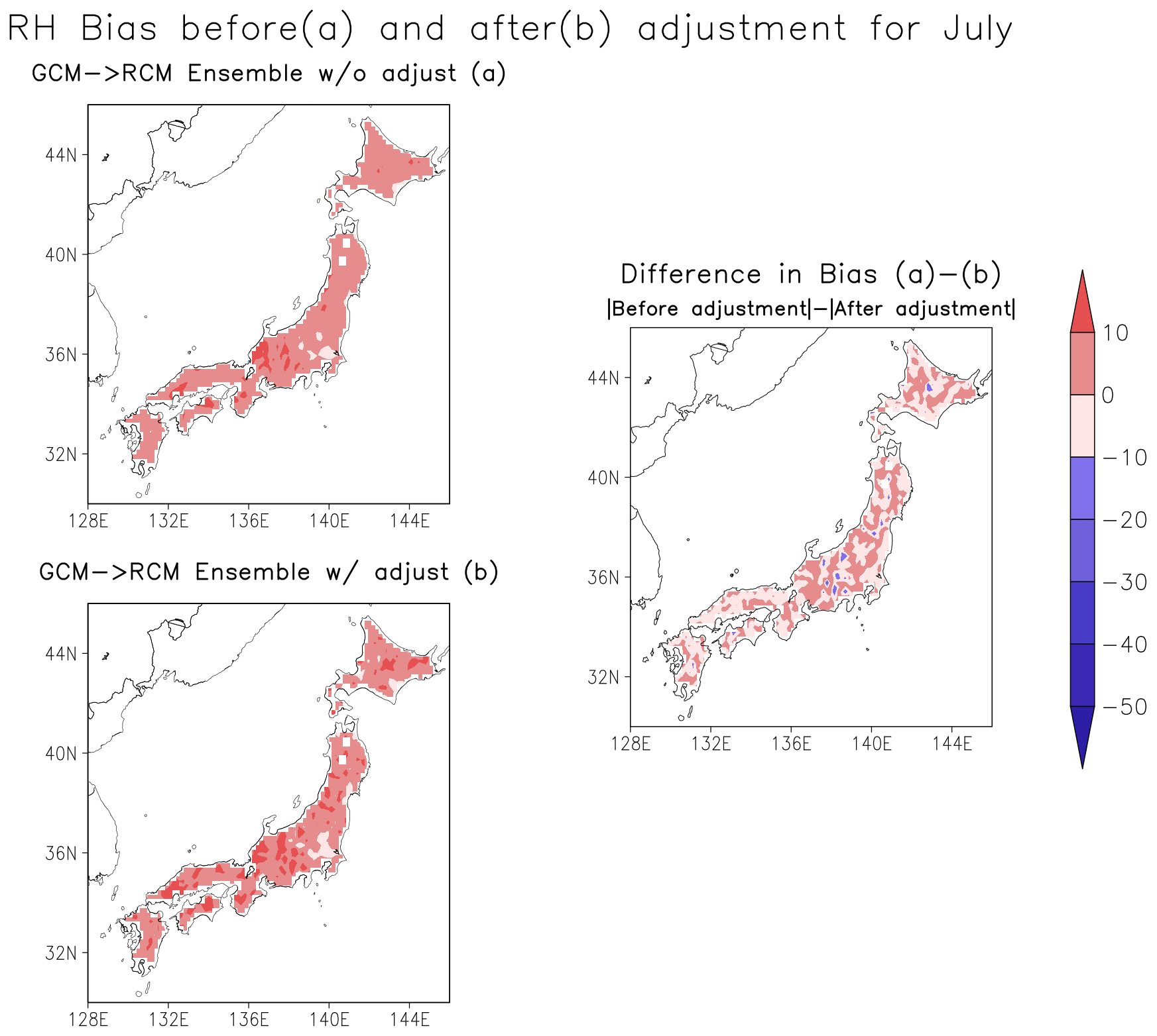
Figure 4 RH bias before (a) and after (b) applying adjustment factor to GCM forced RCM ensemble simulations.

It also points out that the bias reductions are also based on removing surface dependence of air temperature and relative humidity; however, it does not affect the bias originating with structural differences in each model. Since the structural difference arises from different physical schemes used in the model framework, the retained bias is also related to the precision of physical schemes in resolving atmospheric conditions.

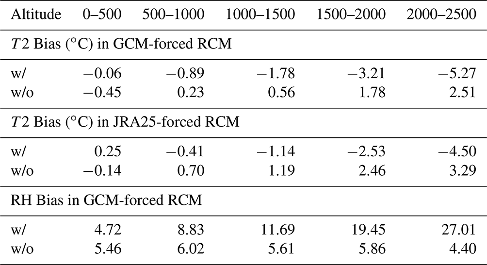
Table 1 Bias at different altitude ranges (in meters) before (w/o) and after (w/) bias adjustment.

Added value assessment contributes to our understanding of the model uncertainties. It highlights areas where models may excel and areas where they may fall short. In our study, we investigated altitudinal variation added value (Fig. 5). Positive added values are present before adjustment, indicating additional information provided by RCM. After the adjustment, RCMs still provide additional information but at a lesser magnitude. On the other hand, at lower altitudes, negative added values before adjustment are improved after adjustment (Fig. 5b, d), highlighting the combined skill of bias adjustment and RCM. It also indicates that the GCM biases have become comparable to RCMs after that adjustment, leading to significant improvement in values added at lower.

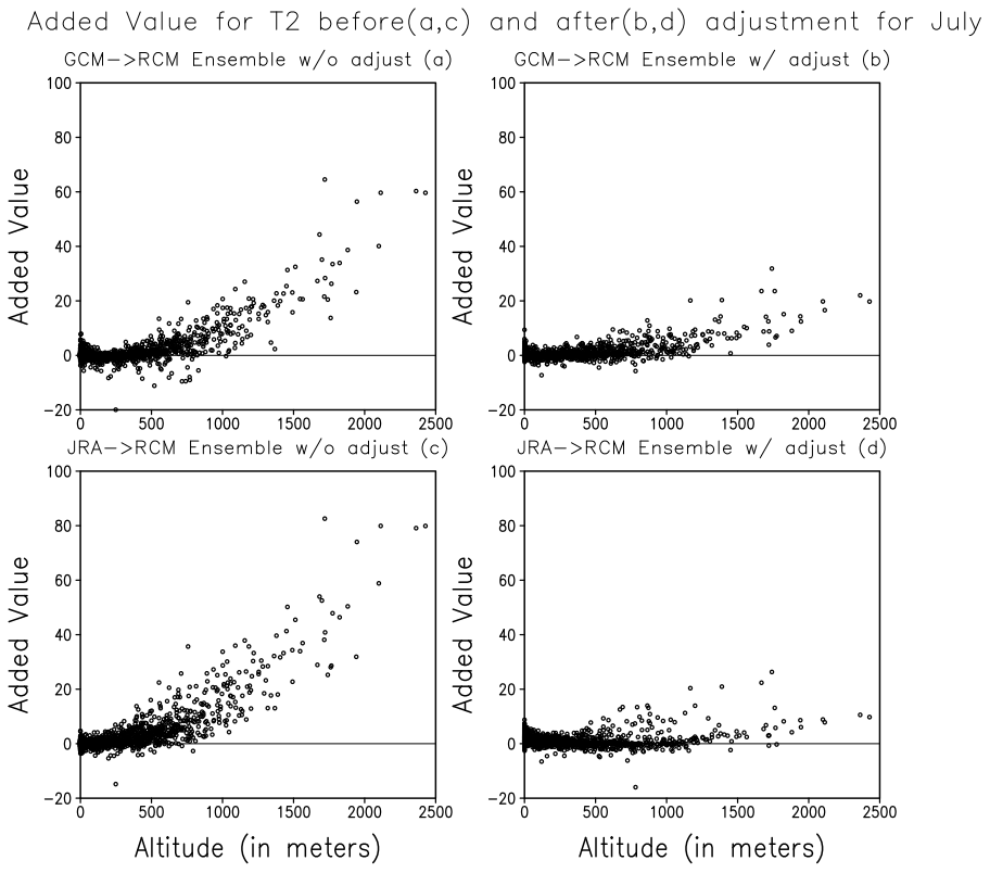
Figure 5 Comparison of added value in T2 in GCM forced (a, b) and JRA25 forced (c, d) ensemble simulations.

Similar to the estimation of added values for air temperature, added values for relative humidity were also calculated. The added bias in RH after adjustment at higher altitudes has impacted the overall representation of added values. The magnitude of added bias in the GCM ensemble was significantly larger than in RCMs, indicating strong positive added values (Fig. 6a, b).

Figure 6 Comparison of added value in RH in GCM forced RCM ensemble simulations.

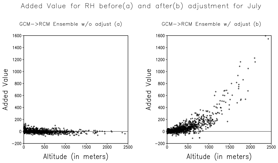
In our study, the efficiency of Multi-Variable Bias Adjustment varied from variable to variable. In the case of air temperature, warm biases were reduced, but it retained a cold bias after the adjustment. As Multi-Variable Bias Adjustment is solely based on topography adjustments, the bias reductions are also based on removing the biases arising from orography representation in the climate model; however, it does not affect the bias originating from the structural differences in each model. Dissimilarity in physical schemes applied in each model to simulate surface-dependent convective processes would still contribute to total bias. In the added values, large added biases in GCMs after the adjustment resulted in strong positive added values, indicating that the interpretation of this type of added value might be related to the magnitude of the added bias and not reductions in biases after the adjustment.

4 Conclusions

The multi-variable bias adjustment shows a substantial reduction in T2 bias after the adjustment. Noticeably, the strong bias over the complex topography of central and northern Japan was reduced. Furthermore, the value added by the RCMs for T2 shows reduction at higher altitudes. In addition, the more substantial negatives observed over lower altitudes were improved to weaker negatives. On the other hand, the assessment of RH shows bias reductions over lower altitude areas (< 500–700 m); however, the bias is retained over mountainous areas. Preserving inter-variable dependence is prominent for compound event assessment; however, in the case of a climate model, retaining that dependence would be challenging because of inherent biases. As highlighted earlier, the bias adjustment based on topographical adjustments reduces the effect of underlying topography but does not affect the bias originating from the structural differences inherent to the model. Therefore, another justification for amplified RH bias could be the combined effect of bias propagated from the parent model to RCMs, the inter-variable (while estimating RH from T2) bias transition, and the limitation of the bias adjustment method in considering the bias related to structural uncertainties. Overall, we observe bias reduction over low altitudes. The advantage of considering topography-based post-processing is it is independent of observational data, allowing its application when observational records are limited or lacking over a particular region (e.g., Tibetan plateau) or for long-term assessments (e.g., pre-industrial, future projections). Hydrological studies could also benefit from this approach, as processes such as rainfall run-off are highly sensitive to the terrain; however, they remain to be explored in future studies.