the Creative Commons Attribution 4.0 License.
the Creative Commons Attribution 4.0 License.
 | 19 Apr 2024
Hydraulic Analysis of the Marikina River Floodplain During Typhoon Vamco using Numerical Modelling
Jonathan S. Serrano
Eugene C. Herrera
Kensuke Naito
Typhoon Vamco in 2020 costed the Philippines over PHP 19 billion in damages. One of the heavily affected floodplains is the Marikina River floodplain. Discharges of up to 2582 m3 s−1 along Marikina River were noted. This is the strongest flashflood incident in the area after Typhoon Ketsana in 2009. This study aims to investigate the hydraulics of flood development within the Marikina River floodplain during Typhoon Vamco using numerical modeling. The hydraulic model in HEC-RAS utilized a 1 m LIDAR DTM, calibrated discharges from a hydrologic model and water levels as upstream and downstream boundary conditions, respectively, and a rain-on-grid input. Results showed a max inundation area of ∼ 75 km2 and flood depths of up to 4 m which accounts for the damages in some municipalities and cities in Metro Manila and Rizal Province. Model validation showed the simulated peak level (11.31 m a.s.l.) to be only 1.0 % lower than the peak observed water level (11.43 m a.s.l.). Model results can be used for measures to minimize risk and damages.
- Article
(4319 KB) - Full-text XML
- BibTeX
- EndNote


Around 80 % of the natural disasters occurring in the Philippines are attributed to hydrometeorological events like typhoons and floods (Jha et al., 2018). These events cause a lot of socioeconomic damages. About twenty typhoons enter the Philippine Area of Responsibility (PAR) each year, with about eight to nine of these making landfall, and about five are considered destructive based on the Asian Disaster Reduction Center (Santos, 2021). On 26 September 2009, Typhoon Ketsana or Tropical Storm Ondoy struck parts of Luzon. Around 455 mm of rains were poured in 24 h, although about 347 mm of these poured in just 6 h. Ondoy caused 464 fatalities and costed more than PHP 11 billion (NDCC, 2009) in damages. A more recent typhoon, Vamco a.k.a. Typhoon Ulysses, made landfall on 11 November 2020 and heavily struck parts of Luzon. Vamco poured 356 mm of rains in 24 h, killing 101 people and costing over PHP 19 billion (NDRRMC, 2021) in damages. Communities beside Marikina and Pasig Rivers were highly affected due to downpour over Marikina River Basin. Flood risk is extremely high in the said areas due to the size of the Marikina River Basin and due to the highly urbanized communities within Metro Manila and Rizal Province. Damages to infrastructure and agriculture brought about by Vamco in Metro Manila alone were around PHP 717 million (NDRRMC, 2021). The River Basin and its floodplain are also highly monitored, which makes it a good site for flood modeling studies. The purpose of this study is to assess the hydraulics of flood development (i.e. flood depths, inundation extents, and timing of flood propagation, etc.) within the floodplain of Marikina River Basin using numerical modeling and to know what solutions can be done to minimize the flood risk. The Hydrologic Engineering Center (HEC) tools of the US Army Corps of Engineers (USACE) were used to assess the flood development of Typhoon Vamco.
2.1 Study site
The Marikina River Basin has a catchment area of around 546 km2. It is located at the southern part of Luzon, less than 5 km northwest of Laguna Lake, and around 9 km east of Manila Bay. About 90 % of the basin is in the mountainous province of Rizal while the rest and more downstream section is in the highly urbanized Metro Manila. The whole study site is comprised of the Marikina River Basin, along with Manggahan Subbasin (∼ 85 km2) and Taguig Subbasin (∼ 43 km2) which both drain to Laguna Lake. The two subbasins are also part of the floodplain of Marikina River due to the complex river network in the floodplain. The Marikina River Basin has a dendritic drainage system, with its vast network of streams converging into the Upper Marikina River. The Upper Marikina River diverges into the Lower Marikina River and the Manggahan Floodway, which is a man-made channel constructed to divert flows to Laguna Lake before eventually discharging into Pasig River during storm events. The Lower Marikina River diverges into Pasig River to the west which naturally discharges to Manila Bay and into Napindan Channel to the east which leads to Laguna Lake. Along the Upper Marikina River is the Sto. Niño Water Level Monitoring Station (WLMS), which is considered a crucial point for the models in this study. Figure 1 shows the study site, where both hydrologic and hydraulic model domains are delineated; its location within Luzon, which is the largest island in the Philippines; and a closer look at the river system within the Marikina River floodplain.
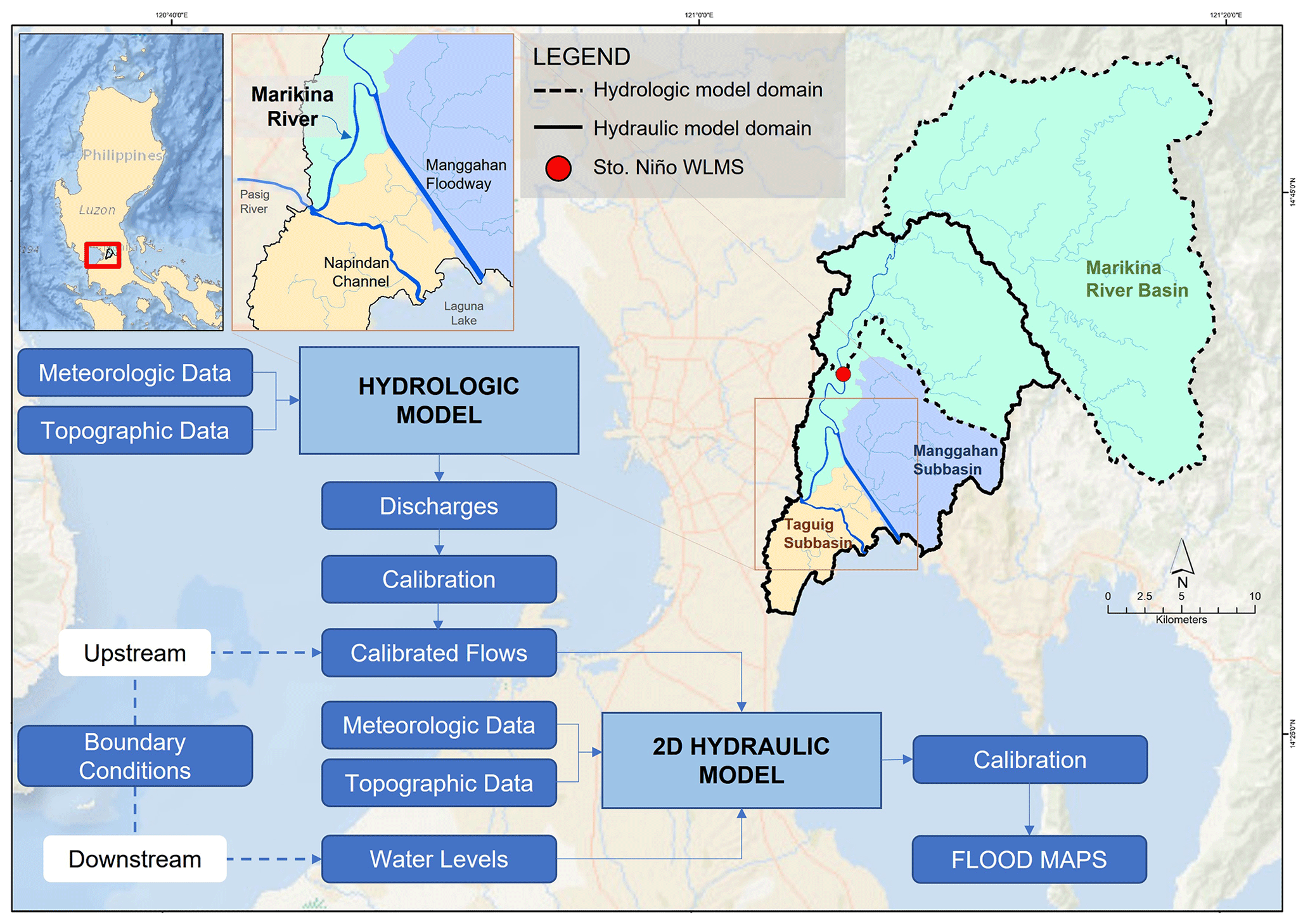
Figure 1Study site, model domains, and methodological framework (Ocean Basemap Source: ESRI).
2.2 Methodological framework
The flood model consists of both a hydrologic and a hydraulic model. The hydrologic model transforms the rainfall over the more upstream areas of the Marikina River Basin into runoff along the Upper Marikina River. The model's extent is set such that the outlet is set at the Sto. Niño WLMS. Discharges available at this station were used to calibrate the hydrologic model. After calibration, flows at a more upstream segment of the Upper Marikina River were extracted from the model and were used as upstream boundary condition for the 2D hydraulic model. Aside from these flows, water levels at the lake and at the confluence of Pasig River and Marikina River were used as boundary conditions. The hydraulic model results to flood maps at any timestep within the simulation period. This model was calibrated so that the simulated water levels at Sto. Niño WLMS will be as close as possible to the observed water levels at that section. Once calibrated, flood maps were generated and flood depths, inundation areas, and flood volumes were extracted. Both secondary meteorologic and topographic data were used in the hydrologic and hydraulic models. The methodological framework is also shown in Fig. 1.
2.3 Data
2.3.1 Terrain
Digital Elevation Models (DEM) were used as terrain input for both hydrologic and hydraulic models. Interferometric Synthetic Aperture Radar – Digital Terrain Model (IFSAR – DTM) with 5 m resolution (NAMRIA, Philippines, 2013) was used for the hydrologic model while Light Detection and Ranging (LIDAR) DTM with 1 m resolution was used for the hydraulic model. Bathymetry of main rivers were included in the hydraulic model for more accurate computations of water depths and velocities. Since bathymetric points were only available for the reaches of Lower Marikina River, Manggahan Floodway, and Napindan Channel, bathymetric data along the Upper Marikina River was extrapolated using the elevations at the confluence of Manggahan Floodway and Marikina River, and the slope of the water level surface along the Upper Marikina River as reflected by the LIDAR DTM (assumed equal to the bed slope).
2.3.2 Land and soil covers
The 2015 Land Cover Map from the National Mapping and Resource Information Authority (NAMRIA, Philippines, 2015) and soil data from the Food and Agriculture Organization (FAO-UNESCO, 1981) were used to determine SCS curve numbers for the hydrologic model. The same land cover map was used for Manning's N values in the hydraulic model.
2.3.3 Meteorologic data
The meteorologic data used for both models were hourly rainfall datasets. A single time-series data was used for each model, with each time-series data comprising a combination of point rainfall data that would yield the highest rainfall volume. The point rainfall datasets were from the ground-based weather gauges in the vicinities of respective model domains. Rainfall volume was maximized to attain enough flood volume both for the hydrologic and hydraulic models, since it was seen that using a spatially averaged rainfall data prepared using Thiessen weights yielded an underestimated flood volume. The data used for the hydrologic model were from the following gauges: Aries, Boso-Boso, Mt. Campana, Mt. Oro, and Nangka. For the hydraulic model, Mt. Campana was removed, while the gauges of Napindan and Science Garden were added to the list.
2.3.4 Water levels and discharges
Rating curve-derived discharges at Sto. Niño WLMS were used to calibrate the hydrologic model. Meanwhile, the water levels at the same station were used to calibrate the hydraulic model. Other secondary water level data were used as downstream boundary conditions for the hydraulic model.
2.4 Model set-up
2.4.1 Hydrologic model
HEC-HMS (Hydrologic Modeling System) was used as the hydrologic modeling platform. The model domain was first delineated into 43 subbasins and 21 reaches. The methods chosen for the model are as follows: SCS Unit Hydrograph for the rainfall-runoff transformation; SCS Curve Number for infiltration loss; Simple Canopy and Simple Surface for the stored water in canopies and surfaces respectively; Constant Monthly for the baseflow; and Kinematic Wave method for the river routing of flows. The simulation period used for the hydrologic model was from 10 November 2020, 00:00:00 LT to 13 November 2020, 23:00:00 LT. This three-day period was enough to include a warm-up for the model, as well as enough time for flood wave attenuation after peak discharge occurs at the outlet. Computation time interval was set to one minute. The main parameter adjusted for calibration was the lag time in the SCS Unit Hydrograph method. Initial values for this input were computed using watershed parameters obtained from topographic data.
2.4.2 Hydraulic model
A 40×40 m grid was set up over the 2D flow area in HEC-RAS (River Analysis System). A Manning's N map was also set over the same area. Boundary condition lines were placed in respective positions: at the upstream end of the Upper Marikina River within the model domain; at the confluence of Marikina River and Napindan Channel, which is at the west boundary of the model extent; and at the edge of the model domain adjacent to Laguna Lake at the southeast. Simulation period was set from 11 November 2020, 02:00:00 LT to 13 November 2020, 23:00:00 LT. The diffusion wave equation was utilized to maintain model computation stability at five-second computation time interval. Adjustments of the Manning's N values of channels were made until the closest fit between the observed and simulated water levels at Sto. Niño WLMS were attained.
3.1 Flood development
The inundation area was determined for every two hours starting from the 11 November 2020, 03:00:00 LT timestep, and for the initial timestep at 11 November 2020, 02:00:00 LT to see the flooding brought about solely by the initial conditions in the model. The inflow hydrograph, shown in Fig. 2, peaks at 2126 m3 s−1 on 12 November 2020, 09:00:00 LT. Maximum flood volume also occurs at this timestep. However, maximum inundation in terms of area (∼ 75 km2) was attained four hours prior to this, signifying that flood extent is maxed earlier than occurrence of peak discharge and starts to decline even before flood depths increase in more flood prone areas. Figure 2 shows the rainfall hyetograph, upstream discharges (i.e. the inflow hydrograph to the hydraulic model), the inundated area within the floodplain, along with the timing of peak values.
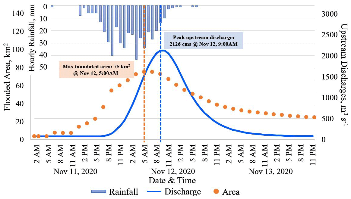
A notable increase in the flooded areas in km2 can be seen from the ninth to eleventh data points (11 November 2020, 17:00:00, 19:00:00, and 21:00:00 LT; 22, 36, 54 km2 respectively). The start of this period coincides with the time when inflow discharges start increasing from its baseflow value of 75 m3 s−1. Rainfall also starts to increase significantly in the said period. Results show it took 16 h of continuous raining within the floodplain before maximum inundation area was attained (starting from 11 November 2020, 13:00:00 LT), and another 19 h for the flooded area to decrease by 50 %.
3.2 Maximum flood depths
The average maximum flood depths per land cover type as well as per barangay were extracted. Max flood depths per land cover type were noted to know the extent of damage in built-up areas and other types in which damage from floods may have economic implications such as grasslands and agriculture. Average max depths in built-up areas, agricultural lands, and grasslands were found to be 0.8, 2.1, and 1.3 m, respectively. Average max flood depth over built-up areas was the lowest among all land cover types within the floodplain since it covers most of the model domain. Rain-induced local ponding in some areas which are much shallower than riverine floods tend to decrease the average depth. The most heavily flooded barangays based on the max flood depth map were Dulong Bayan I (4.00 m), Guitnang Bayan I (2.97 m), Concepcion Uno (2.22 m), Guinayang (2.20 m), and Jesus de la Peña (2.18 m). Figure 3 below shows the resulting max flood depth map and the five most heavily flooded barangays in terms of flood depths.
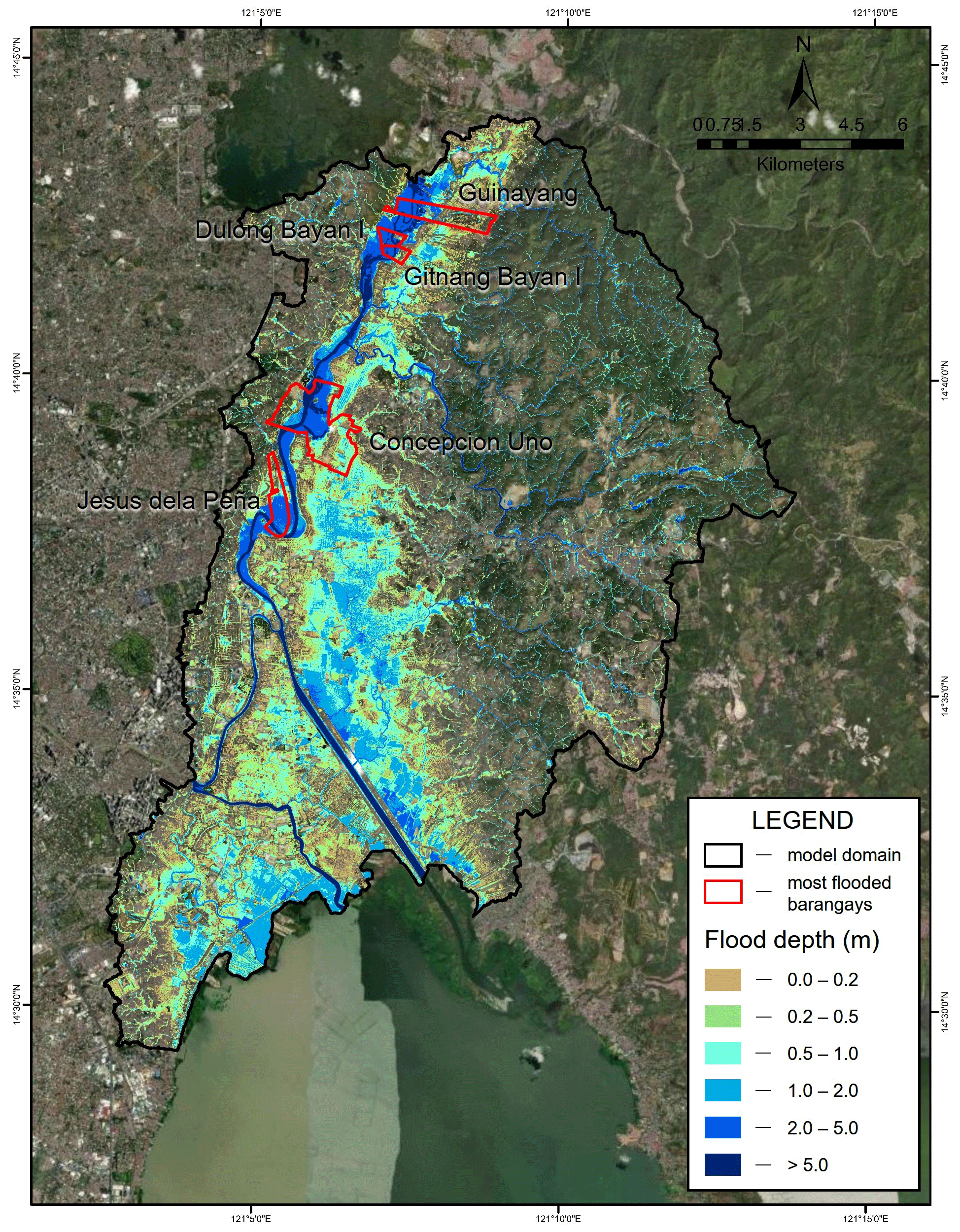
Figure 3Maximum flood depth map and the five most flooded barangays (World Imagery Basemap Source: ESRI).
3.3 Model calibration
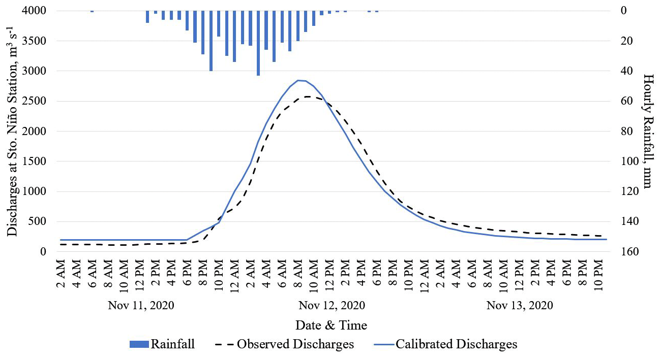
For the hydrologic model, adjusting the lag time of the subbasins among other watershed parameters resulted to a Nash Sutcliffe efficiency (NSE) of 0.97 and a percent bias (PBIAS) of 1.7. These values are classified as having “very good” model performance rating (Moriasi et al., 2007). However, simulated peak discharge (2854 m3 s−1) was 10.5 % higher than the observed (2582 m3 s−1) at Sto. Niño. The simulated peak discharge also occurred one hour ahead (12 November 2020, 09:00:00 LT) of the observed. Further calibration and input data reassessment can minimize this gap. The hydrologic model calibration plot is shown in Fig. 4.
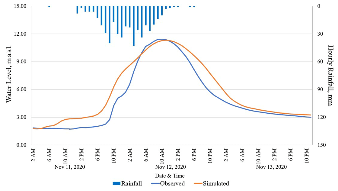
For the hydraulic model, adjusting the Manning's N of main channels to 0.035 yielded the nearest peak water level in terms of both depth and timing. This resulted to an NSE of 0.88, with the simulated level (∼ 11.31 m a.s.l.) being only 1 % lower than the observed (∼ 11.43 m a.s.l.). This peak occurs one hour later in the simulation (12 November 2020, 11:00:00 LT) than the observed. The hydraulic model calibration plot is shown in Fig. 5.
This figure translates to a time to peak of ten1 hours. This is the length of time between the centroid of the rainfall hyetograph and the peak discharge. More sense or implication can be deduced upon looking at the cumulative rainfall of the data used. Results showed that 20 h of continuous rainfall that accumulates to ∼ 230 mm, and/or 24 h accumulating to ∼ 350 mm of rains can produce the same inundation caused by Typhoon Vamco. These values, along with information on flood extent can give lead times of ten and/or six hours respectively before peak flood volume occurs. Further development and calibration of both models can still improve the results. Continuous datasets of water levels and discharges of another storm event can also be used for validation. Such flood models can be the key to flood risk mitigating solutions.
3.4 Simulation-based recommendations
From the results, it can be recommended to authorities to shift the focus from water level monitoring to rainfall monitoring as this would give a lot more lead time for evacuation. It is also highly recommended to use updated flood maps in determining safe evacuation sites. Regularly updating flood risk maps may also be helpful since lots of factors can alter the topography which play a crucial role in the flood development during storm events.
This study showed the effectiveness of using numerical models to investigate the flood development of a strong typhoon such as Typhoon Vamco. A coupled hydrologic model (HEC-HMS) and hydraulic model (HEC-RAS) that yielded an NSE of 0.97 for discharge hydrographs and 0.88 for stage hydrographs respectively, implies the nearness of the model results to that which occurred during Typhoon Vamco. A difference of 1 % in the peak water level at Sto. Niño WLMS and the one-hour difference in time-to-peak of simulated and observed values also imply a certain level of accuracy. Average max flood depths and timing of flood extents as well as flood volumes for different timesteps were determined. This study can help assess already existing flood control plans in the area, with the overall objective of minimizing flood risk and damages in the future.
Only processed data directly used for the final version of the model are available upon request. Raw data are to be gathered from the agencies from which the authors collected such datasets.
ECH conceptualized the study upon the request of a stakeholder for a research project. JSS set up and simulated the models, conducted the extraction, analysis, and documentation of model results upon the supervision of ECH. JS wrote the draft and edited it based on the review done by ECH. KN also reviewed the abstract and supported the overall study for its submission to the ICFM9 conference.
At least one of the (co-)authors is a guest member of the editorial board of Proceedings of IAHS for the special issue “ICFM9 – River Basin Disaster Resilience and Sustainability by All”. The peer-review process was guided by an independent editor, and the authors also have no other competing interests to declare.
Publisher's note: Copernicus Publications remains neutral with regard to jurisdictional claims made in the text, published maps, institutional affiliations, or any other geographical representation in this paper. While Copernicus Publications makes every effort to include appropriate place names, the final responsibility lies with the authors.
This article is part of the special issue “ICFM9 – River Basin Disaster Resilience and Sustainability by All”. It is a result of The 9th International Conference on Flood Management, Tsukuba, Japan, 18–22 February 2023.
This research was supported by the Project for Development of a Hybrid Water-Related Disaster Risk Assessment Technology for Sustainable Local Economic Development Policy Under Climate Change in the Philippines (HyDEPP-SATREPS) of the Japan International Cooperation Agency (JICA) and Japan Science and Technology Agency (JST); and the Department of Science and Technology (DOST) and DOST Philippine Council for Industry, Energy and Emerging Technology Research and Development (DOST-PCIEERD) through the project Eco-System Modelling and Material Transport Analysis for the Rehabilitation of Manila Bay (e-SMART) under the IM4ManilaBay Program.
This research has been supported by the Science and Technology Research Partnership for Sustainable Development (grant no. JPMJSA1909) and the Department of Science and Technology, Philippines (grant no. Eco-System Modelling and Material Transport Analysis for the Rehabilitation of Manila Bay (e-SMART) Project).
This paper was edited by Mohamed Rasmy and reviewed by two anonymous referees.
FAO-UNESCO: Digital Soil Map of the World, FAO-UNESCO [data set], https://www.fao.org/soils-portal/data-hub/soil-maps-and-databases/faounesco-soil-map-of-the-world/en (last access: 18 March 2024), 1981.
Jha, S., Martinez, A., Quising, P., Ardaniel, Z., and Wang, L.: Natural Disasters, Public Spending, and Creative Destruction: A Case Study of the Philippines, ADBI Working Paper 817, https://doi.org/10.2139/ssrn.3204166, 2018.
Moriasi, D. N., Arnold, J. G., Van Liew, M. W., Bingner, R. L., Harmel, R. D., and Veith, T. L.: Model Evaluation Guidelines for Systematic Quantification of Accuracy in Watershed Simulations, T. ASABE, 50, 885–900, https://doi.org/10.13031/2013.23153, 2007.
NAMRIA, Philippines: IFSAR DEM, Photogrammetry Division, Mapping and Geodesy Branch [data set], https://namria.gov.ph/Files/Request for IFSAR and LIDAR Data, Orthoimage, Orthophoto and Aerial Photographs.pdf (last access: 18 March 2024), 2013.
NAMRIA, Philippines: Land Cover Map, Resource Data Analysis Branch, 2015.
National Disaster Coordinating Council (NDCC): SitRep 48 on TS “Ondoy” and Typhoon “Pepeng”, Report, https://reliefweb.int/attachments/b5da56c0-e8de-30ea-9352-f59e4948cd61/D2F7A40978978E214925766C001B455A-Full_Report.pdf (last access: 18 March 2024), 2009.
National Disaster Risk Reduction and Management Center (NDR- 15 RMC): SitRep 29 re Preparedness Measures and Effects for Typhoon “ULYSSES” (I.N. VAMCO), Report, https://reliefweb.int/attachments/c81781d2-633e-3fae-bd53-82d7517e94dd/SitRep_no_29_re_TY_Ulysses_as_of_13JAN2021.pdf (last access: 18 March 2024), 2021.
Santos, G. D.: 2020 tropical cyclones in the Philippines: A review, Tropical Cyclone Research and Review, 10, 191–199, https://doi.org/10.1016/j.tcrr.2021.09.003, 2021.
considering hydrograph from the simulation