Spatially distributed calibration of a hydrological model with variational optimization constrained by physiographic maps for flash flood forecasting in France

This contribution presents a regionalization approach to estimate spatially distributed hydrologic parameters based on: (i) the SMASH (Spatially distributed Modelling and ASsimilation for Hydrology) hydrological modeling and assimilation platform (Jay-Allemand, 2020; Jay-Allemand et al., 2020) underlying the French national flash flood forecasting system Vigicrues Flash (Javelle et al., 2019); (ii) the variational assimilation algorithm from (Jay-Allemand et al., 2020), adapted to high dimensional inverse problems; (iii) spatial constraints added to the optimization problem, based on masks derived from physiographic maps (e.g., land cover, terrain slope); (iv) multi-site global optimization, which targets multiple independent watersheds. This method gives a regional estimation of the spatially distributed parameters over the whole modeled area. This study uses a distributed rainfall-runoff model with 4 parameters to calibrate, with a spatial resolution of 1×1 km² and a 15 min time step. Performances of the calibrated hydrological model and the parameters robustness are evaluated on two French study areas with 20 catchments in each, in spatio-temporal extrapolation based on cross-validation experiments over a 12-year period. Several spatial regularization strategies are tested to better constrain the high dimensional optimization problem. The model parameters are calibrated based on the Nash-Sutcliffe Efficiency (NSE) computed for multiple calibration basins in the study area. Results are discussed based on the Nash-Sutcliffe Efficiency and the Kling-Gupta Efficiency criteria obtained on calibration and validation catchments for two subperiods of 6 years. Further work aims to improve the global search of prior parameter sets and to better balance the adjoint sensitivity with respect to the spatial constraints resolution and catchment characteristics. This will ensure a better consistency of simulated fluxes variabilities and enhance the applicability of the regionalization method at higher spatial scales and over larger domains.

1 Introduction

The estimation of storage and fluxes in surface hydrology is an essential scientific question related to major socio-economic issues as extreme floods and droughts forecasting, especially with the undergoing climate change. In order to better predict flash floods and reduce their potentially devastating impact, warning systems have been developed or are currently under development (Gourley et al., 2017; Javelle et al., 2016). In this context, advanced spatially distributed modeling tools are critically needed to generate reliable and skillful local forecasts. These models take into account the spatial variability of the catchment properties and of the forcing inputs (e.g., rainfall) to produce discharge predictions at ungauged locations. Nevertheless, hydrological modeling remains a challenging task because of limited observations of physical processes and modeling uncertainties, and internal storage fluxes are tinged with uncertainties.

Whatever their status and complexity, hydrological models are most often calibrated and validated using integrative discharge time series at the outlet of a catchment (e.g. Sebben et al., 2013). However, due to a potentially significant number of cells or subcatchments involved in distributed models, the calibration process has to deal with overparameterization and equifinality (uniqueness) issues. In particular, given the spatial sparsity of constraining discharge observations, hydrological modeling is faced with the challenge of producing predictions at ungauged locations based on the regionalization of the hydrological model parameters. Despite the overparameterization problem in spatially distributed modeling, the contribution of e.g. Jay-Allemand et al. (2020) and Jay-Allemand (2020) showed promising results for estimating the spatial variability of the distributed parameters within a given catchment using only downstream discharge observations. However, providing better spatial constrains on the estimated parameters patterns, within and outside the calibration catchments in a regionalization perspective, remains a challenge.

Different regionalization strategies have been proposed in hydrology. Some methods search for relations between the model parameters and physical descriptors (Seibert, 1999). Others methods explore regionalization schemes based on the spatial or physical proximity (e.g. Odry and Arnaud, 2017; Parajka et al., 2005). These methods have many requirements: (1) reliable parameters have to be identified on gauged catchment; (2) hydrological relations between gauged and ungauged catchments must exist; (3) model parameters should have a physical meaning. Unfortunately, these requirements are not always satisfied. To better constrain regionalization over large domains, promising regional calibration results of Samaniego et al. (2010), Poncelet (2016), Mizukami et al. (2017), and Beck et al. (2020) are based on the Multiscale Parameter Regionalization (MPR) upscaling and pre-regionalization scheme of Samaniego et al. (2010), which enables to account for various physiographic and climatic descriptors. It consists in imposing a mapping between fine scale descriptor maps and model parameter maps prior to regional optimization. Nevertheless, in all those studies, the mapping parameters are optimized as spatially uniform with classical optimization algorithms limited to low dimensional inverse problems.

In a regionalization perspective, we extend the distributed calibration approach developped by Jay-Allemand et al. (2020), which is adapted to high dimensional hydrological inverse problems. Our regional calibration method uses the following elements: (1) a distributed hydrological model; (2) a variational algorithm; (3) the adjoint of the forward model; (4) physical descriptors to constrain the spatial variability of the parameters; (5) a regularization function, required for ill-posed inverse problems (Tikhonov, 1963), adapted to constrain the distributed hydrological model with physical descriptors. Finally, the major difference with others regional calibration approaches lies in the fact that no prior guess based on hypothetical physical meanings of the parameters is required. The descriptors are only used to define classified physiographic maps to constrain the parameter patterns through the control setting or the regularization function.

2 Modeling approach

SMASH is a computational software framework dedicated to Spatially distributed Modeling and data ASsimilation for Hydrology at high resolution, capable to tackle high dimensional inverse problems with variational data assimilation. It underlies the French flash flood warning system called Vigicrues Flash (Javelle et al., 2019).

2.1 SMASH Model

Let Ω⊂ℝ² be a 2D spatial domain, containing single to multipe nested and non-nested catchments, and t>0 be the physical time. A regular lattice 𝒯_Ω covers Ω and D(x) is the drainage plan obtained from terrain elevation processing, with the only condition that a unique point in Ω has the highest drainage area, i.e. the outlet of the largest catchment in Ω. The hydrological model is a dynamic operator ℳ mapping the observed input fields of rainfall and evapotranspiration, denoted $\mathit{P}\left(x,t^{\prime }\right)$ and $\mathit{E}\left(x,t^{\prime }\right)$, $\forall \left(x,t^{\prime }\right)\in \mathrm{\Omega }\times (\mathrm{0},t)$ onto the discharge field Q(x,t) such that:

$$\begin{array}{}\text{(1)}& \begin{array}{rl}Q\left(x,t\right)& =\mathcal{M}\left[\mathit{P}\left(x,t^{\prime }\right),\mathit{E}\left(x,t^{\prime }\right),\mathit{h}\left(x,\mathrm{0}\right),\mathit{\theta }\left(x\right)\right]\\ & \forall \left(x,t^{\prime }\right)\in \mathrm{\Omega }\times \left[\mathrm{0},t\right]\end{array}\end{array}$$

with h(x,t), the N_s-dimensional vector of model states (2D fields), and θ, the N_p-dimensional vector of model parameters (2D fields); θ is also called the control vector in the optimization context.

In this study, we use a parsimonious 4-parameters gridded GR-like hydrological model schematized in Fig. 1. For a given pixel i of coordinates x∈Ω, the proposed model includes three reservoirs 𝒫, 𝒯_r and 𝒯_l of capacity c_p, c_tr and c_tl, to simulate respectively the production of runoff and its transfer within a cell (with two transfer reservoirs). Their stages are respectively denoted h_p, h_tr and h_tl. Given known flow directions, classically obtained from a Digital Elevation Model, the cell-to-cell routing is done with a nonlinear routing reservoir ℛ of capacity c_r. The spatial resolution is set to Δx=1 km and the simulation time step to Δt=15 min corresponding to the space-time resolution of input rainfall and evaporation data, which are assumed to be constant over a given time step Δt. The flow operators, mostly consisting in first order ordinary differential equations, are analytically integrated over a time step, enabling a simple computation of the forward model defined in Eq. (1).

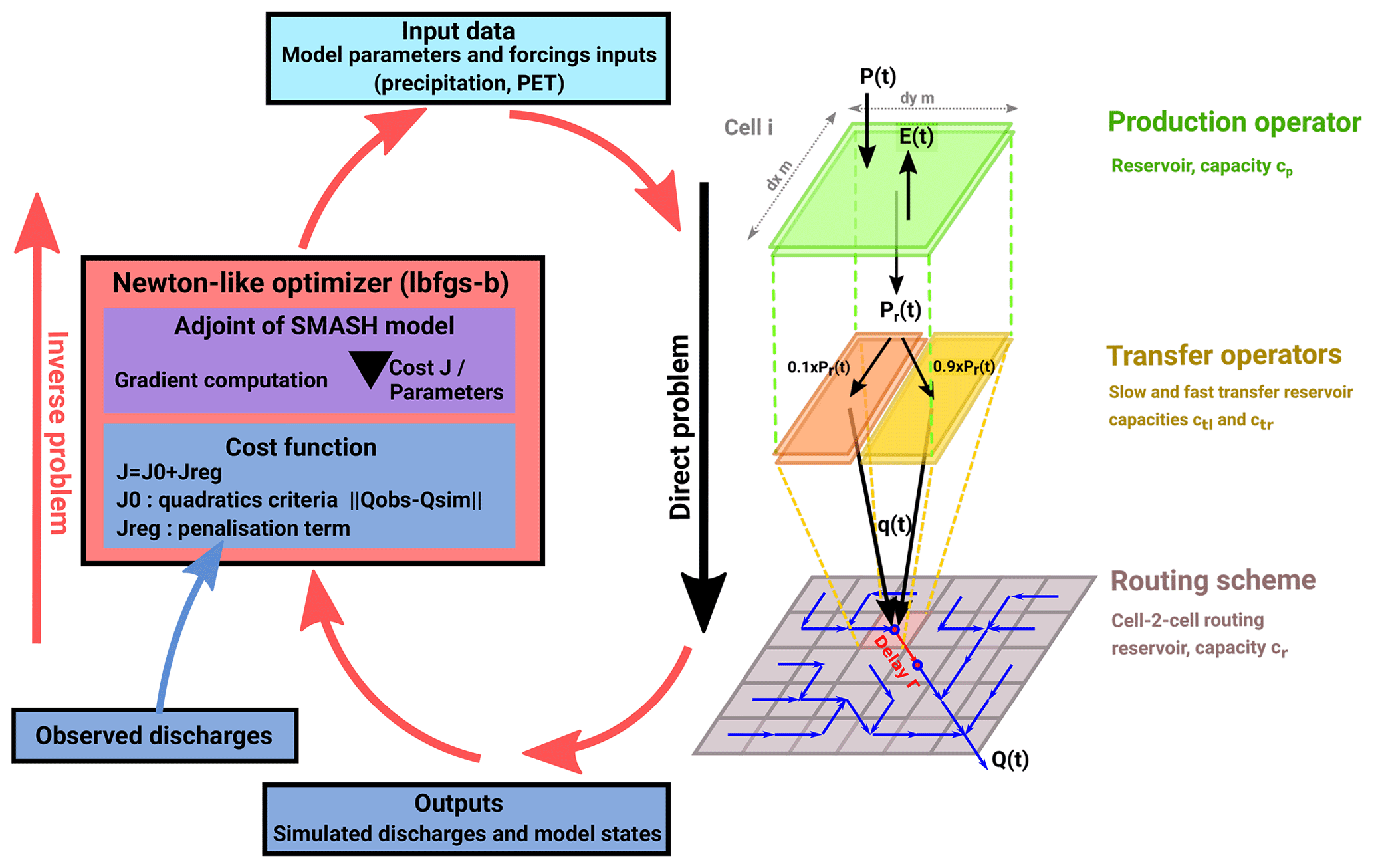
Figure 1 The distributed SMASH hydrological model and the variational algorithm involving the quasi-Newton optimizer lbfgs-b and the adjoint of the forward model.

2.2 Calibration algorithm

In order to better constrain discharge estimates at ungauged locations, the calibration aims to estimate spatially distributed parameters within the calibration catchments as well as outside them. Hence, the parameter vector $\mathit{\theta }\left(x\right)\equiv {\left(c_{\mathrm{p}}\left(x\right),c_{\mathrm{tr}}\left(x\right),c_{\mathrm{r}}\left(x\right),c_{\mathrm{tl}}\left(x\right)\right)}^{\mathrm{T}}$ is of size N_c×N_x, where N_c denotes the number of parameters fields and N_x the total number of cells in Omega Ω, including cells in ungauged areas. Considering tens of cells or more over a given hydrological domain Ω with discharge observations being available only on a limited number of points (i.e. outlets of the gauged catchments), the regional calibration of a spatially distributed θ is a high dimensional and difficult inverse problem.

The adjoint-based variational calibration algorithm developed by e.g. (Jay-Allemand, 2020; Jay-Allemand et al., 2020) and adapted to such hydrological inverse problems, is used in this study and summarized here and in Fig. 1. Given the simulated and observed discharges at gauged cells $x_k\in \mathrm{\Omega },k\in \mathrm{1},..,N_{\mathrm{g}}$, respectively denoted Q_k(t) and $Q_k^{*}\left(t\right)$, we define the objective function as:

$$\begin{array}{}\text{(2)}& J\left(\mathit{\theta }\right)=J_{\mathrm{obs}}\left(\mathit{\theta }\right)+\mathit{\alpha }{J}_{\mathrm{reg}}\left(\mathit{\theta }\right)\end{array}$$

where the observation cost function is $J_{\mathrm{obs}}={\sum }_{k=\mathrm{1}}^{N_{\mathrm{g}}}{j}_k^{*}$. In this study, $j_k^{*}$ is classically defined as 1− NSE, with NSE the Nash-Sutcliffe efficiency (Nash and Sutcliffe, 1970), a quadratic metric that measures the misfit between simulated and observed discharges. Note that the simulated discharge depends on the control vector θ via the hydrological model (Eq. 1). The second term in Eq. (2) is a regularization term weighted by α. Given the ill-posedness of the hydrological calibration problem, classified maps of different physiographic descriptors are introduced to spatially constrain the variability of model parameters fields. For each parameter field of θ, one classified physiographic map is considered to either reduce the control vector into semi-distributed controls or compute a regularization term by class as detailed hereafter.

In order to improve the obtained hydrologic parameter patterns, an additional regularization term is proposed to penalize parameter variability within each physiographic class. Consider for each of the N_c=4 parameters fields ${\mathit{\theta }}_{\mathrm{c}\in [\mathrm{1}..N_{\mathrm{c}}]}\left(x\right)\in \mathit{\theta }\left(x\right)$, a given physiographic map defining a partition of the catchment such that ${\mathrm{\Omega }}_{\mathrm{c}}={\cup }_{k=\mathrm{1}}^{n_{\mathrm{p},\mathrm{c}}}{\mathrm{\Omega }}_{\mathrm{c},k}$ with n_p,c the number of classes in the spatial partition of parameter c. We introduce the following regularization term:

$$\begin{array}{}\text{(3)}& J_{\mathrm{reg}}=\sum _{c=\mathrm{1}}^{N_{\mathrm{c}}}\sum _{k=\mathrm{1}}^{n_{\mathrm{p},\mathrm{c}}}\left(\sum _{i,j}^{i,j\in {\mathrm{\Omega }}_{\mathrm{c}},k}{\displaystyle \frac{\mathrm{1}}{d_{i,j}}}\left|\right|{\mathit{\theta }}_{\mathrm{c}}^i\left(x\right)-{\mathit{\theta }}_{\mathrm{c}}^j\left(x\right)|{|}^{\mathrm{2}}\right)\end{array}$$

where d_i,j is the Euclidean distance between cells i and j. This function, inspired by the classic Tikhonov regularization (Tikhonov, 1963), enables a consistent regularization of the parameters spatial variability within the spatial partitioning Ω_c of each parameter. The weight α is chosen with the L-curve method (Hansen and O'Leary, 1993).

Given the hydrological model defined in Eq. (1), an optimal estimate $\widehat{\mathit{\theta }}$ of the model parameter set is obtained from the condition:

$$\begin{array}{}\text{(4)}& \widehat{\mathit{\theta }}=\underset{{\mathit{\theta }}_{min}\le \mathit{\theta }\le {\mathit{\theta }}_{max}}{\arg min}J\left(\mathit{\theta }\right)\end{array}$$

The optimization is performed with the L-BFGS-B algorithm adapted to high dimension (Zhu et al., 1994). This algorithm requires the gradient of the cost function with respect to the sought parameters, ∇_θJ, which is obtained by solving the adjoint model. The adjoint model has been generated with the automatic differentiation engine TAPENADE (Hascoet and Pascual, 2013) applied to the SMASH source code, which includes the new modeling components and regularization scheme, and has been validated with a standard gradient test. The first guess value $\overline{\mathit{\theta }}$ needs to be defined as a starting point for the optimization process with the regularization term. $\overline{\mathit{\theta }}$ is defined as a spatially uniform global optimum determined with a simple global minimization algorithm from a uniform parameter set, ${\overline{\mathit{\theta }}}^{*}$ (Jay-Allemand et al., 2020). The steepest descent method summarized in (Edijatno, 1991) has been used in this study to determine this uniform first guess value. Note that the semi-distributed calibration of a semi-distributed conceptual model has been investigated in De Lavenne et al. (2019), using a sequential and low dimensional calibration approach involving a regularization strategy accounting for deviation to a priori parameter sets determined with catchment proximity. In the present work, a regularization term penalizing the spatial variability of parameters within physiographic catchment partitioning is introduced in a variational data assimilation algorithm adapted to high dimensional inverse problems; the cost function is global in space and time.

In order to investigate the effects of the proposed regularization term, the following calibration strategies are compared:

• a spatially uniform calibration (denoted U), where the control vector considered constant in space (hence ${\mathit{\theta }}_{\mathrm{U}}\left(x\right)\equiv \overline{\mathit{\theta }}$ reduced to 4 unknowns) is sought with the simple steepest descent algorithm from e.g. (Edijatno, 1991); this uniform calibrated parameter set ${\widehat{\mathit{\theta }}}_{\mathrm{U}}$ is used as the first guess value in the three subsequent calibration processes;

• a distributed calibration (denoted D), with a spatially distributed control θ_D(x), i.e. with free parameters in each cell within the gauged catchments used for calibration; the first guess values (from the uniform calibration) give parameter estimates for all grid cells outside of the gauged catchments;

• a semi-distributed calibration (denoted SD), with a semi-distributed control θ_SD(x) spatially constrained by classified physiographic maps over the whole domain, hence with one spatially uniform free parameter for each class of the physiographic mask relative to the model parameter;

• a distributed-regularized calibration (denoted DR), with a fully distributed control θ_DR(x) since the physiographic regularization from Eq. (3) (based on the same physiographic masks as in the SD calibration) is used in this case as a weak regionalization constrain over the whole domain.

In fact, in the optimization process, the observation cost function is only sensitive to the parameter values of the cells within the gauged catchments used for calibration. However, the regionalization effect stems from the proposed classified physiographic maps either through the semi-distributed control setup for the SD case or from the regularization term in the DR case.

3 Data and experimental setup

The calibration strategies are evaluated over two study areas with 20 gauged basins in each (see Fig. 2): (i) a Northern area in the Burgundy region, (ii) a Southern area in the Ardeche region. These 40 gauged basins, with catchment areas ranging from 25 to 768 km², have been split up in 2 subsets for cross-validation purposes: 28 basins for calibration and 12 basins for validation (5 nested and 7 neighboring catchments). The selection of catchments is based on the availability of long time series with high quality of observed flow and limited anthropogenic impacts. The choice of the localization of the calibration/validation and nested/disjoint catchments is arbitrary.

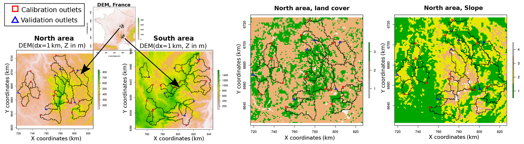
Figure 2 On the left side, catchment boundaries for the North and South study areas, with red squares for the calibration outlets (14 for each area) and blue triangles for the validation outlets (6 for each area). On the right side, the physiographic partitioning relative to the descriptors of land cover and slope for the Northern area.

The SMASH model runs on a 1×1 km² grid resolution at a 15 min time step forced by: (i) observed rainfall grids based on hourly ANTILOPE J+1 radar-gauge rainfall reanalysis (Laurantin, 2013; Champeaux et al., 2009), which have been disaggregated using the temporal distribution of 15 min PANTHERE radar-gauge rainfall estimates available in real-time (both gridded products from Météo-France); (ii) PET estimates based on the Oudin formula and the temperature data from SAFRAN reanalysis produced by Météo-France on a 8×8 km².

Several combinations of physiographic descriptors were tested to spatially constrain the parameter calibration using land use, local slope, bedrock type and drainage areas. Results presented in this paper consider: (i) for the c_p production parameter, a 1 km² land use gridded mask with 3 classes derived from CORINE Land Cover (2012 version, https://land.copernicus.eu/pan-european/corine-land-cover, last access: 9 May 2023) (the 3 classes including artificial areas, open spaces with little or no vegetation and water bodies for class 1, agricultural areas for class 2, and forests for class 3); (ii) for the 3 other transfer and routing parameters (c_tr, c_tl and c_r), a 1 km² local slope grid mask with 4 classes (using the threshold values of 0.025, 0.5 and 1.8° for classes 1 to 4) from the Copernicus database (http://land.copernicus.eu/in-situ/eu-dem-derived-products/slope, last access: 9 May 2023). The numbers of classes was chosen so that each catchment is covered by at least two classes and both descriptors have more or less the same number of classes (3 and 4). We are aware that this choice affects the size of the control of the (SD) case.

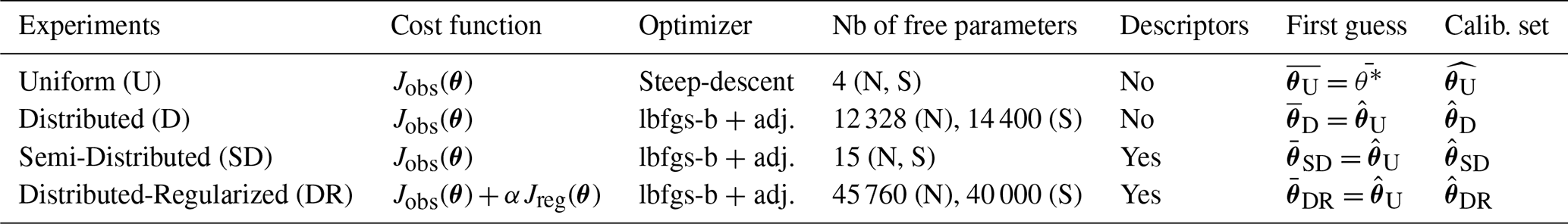
The number of free parameters depends on the study area (Northern and Southern) and the optimization scheme. For the distributed case (D), the number of free parameters is equal to 12 328 (Northern) and 14 400 (Southern), which corresponds to the number of cells inside the gauged catchments times the number of hydrological operators in the forward model. Cells outside the gauged area are not sensitive to the cost function and are therefore not included in the optimization process. For the distributed-regularized case (DR), the number of free parameters is equal to 45 760 (Northern) and 40 000 (Southern), which corresponds to the total number of cells of the domain times the number of hydrological operators in the forward model. Thanks to the regularization function, all domain cells are sensitive to the cost function and are thus included in the optimization process. For the semi-distributed (SD) case, the use of classified physiographic maps for the reduction of the control leads to 15 free parameters, corresponding to the total number of descriptors classes used for all operators. For the uniform (U) case, the control contains only 4 parameters. Table 1 gives a summary description of the configurations of the four calibration experiments.

The parameter bounds for the uniform (U) and semi-distributed (SD) calibration are defined as follows: c_p and c_tr varying between 20 and 1000 mm, c_tl between 20 and 5000 mm, and c_r between 0.1 and 100 min. For the distributed (D) and distributed-regularized (DR) calibrations, the first guess value for each parameter has been used to define the upper bound as ${\mathit{\theta }}_{max}=\mathit{\theta }\left(x_{\mathrm{b}}\right)+\mathrm{3}\times \mathit{\theta }\left(x_{\mathrm{b}}\right)$, the lower bound being equal to 1.

The weight of the regularization, α, was estimated using the L-curve method (Hansen and O'Leary, 1993). The chosen α value varies in the interval of $[\mathrm{7.0},\mathrm{20}.]$ depending on the experiments. It is interesting to mention that, at the end of the optimization, the relative weights $\frac{\mathit{\alpha }{J}_{\mathrm{reg}}\left(\widehat{\mathit{\theta }}\right)}{J_{\mathrm{obs}}\left(\widehat{\mathit{\theta }}\right)}$ remain within the range of [9.0,12.0].

To focus the parameter calibration on high flow conditions, the optimization criterion (NSE) is calculated using only observed flow exceeding one fifth of the flood quantile relative to the 2-year return period. The evaluation scores are all computed with the same thresholding strategy, which leads to lower efficiency score values but a better description of the similarity between observed and simulated discharges for high flow conditions.

Table 1 Characteristics of the four calibration strategies, including the name of the experiment, the cost function, the optimization algorithm, the number of free parameters, the use of the physiographic descriptors, the value of the first guess and the notation of the calibrated parameter set.

The evaluation of the model calibrations consists in analysing the model predictive performance (referred as MPP) using data not involved in calibration (Jay-Allemand et al., 2020). Therefore, the full set of observations $Q^{*}k\left(t\right),k=\mathrm{1},\mathrm{\dots },\mathrm{Ng},t\in (\mathrm{0},T)$ is divided into two complementary subsets: a calibration subset and a validation subset. Since Q^* depends on k (defining the spatial distribution of sensors) and t, we distinguish the temporal validation and spatio-temporal validation, following the split sample test defined by Klemeš (1986). Two 6-year subperiods are defined: P1 from 1 August 2007 to 31 July 2013, and P2 from 1 August 2013 to 31 July 2019. Each subperiod (P1 or P2) is considered as the calibration period while the other period is the validation period. A model warm-up of one year (from August to July preceeding the calibration period) is performed before starting the simulations, one year being long enough to obtain stable model states for these catchments not strongly impacted by snow conditions.

If data from a station is used in calibration, the corresponding catchment is labelled as “calibration catchment”; otherwise it is a “validation catchment”. Both the calibration quality and the MPP in validation are measured using the NSE criterion and the Kling–Gupta efficiency (KGE) criterion (Gupta et al., 2009). The NSE and KGE metrics are computed for high flow conditions only, on the calibration and validation subperiods. The gain in the NSE score is computed for each individual basin as a skill score to evaluate the relative improvement (in terms of NSE) of a given calibration in reference to the benchmark calibration (e.g., the uniform (U) case).

4 Results and Discussions

4.1 Model predictive performances analysis

The distribution of the NSE and KGE values for all 28 calibration catchments (from both study areas) on the calibration and validation periods are plotted on Fig. 3, while results for the 12 validation catchments on the validation period (for spatiotemporal validation) are plotted on Fig. 4. Box-and-whisker plots represent the quartile values, the median value being indicated by the bar within the box and the whiskers extending from the smallest to the largest value.

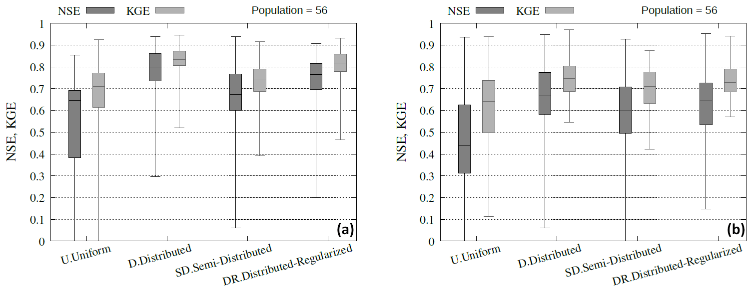
Figure 3 Model performances (NSE and KGE for high flow conditions) at the 28 calibration stations for the four experiments for the 2 calibration subperiods (a) and for the 2 validation subperiods (b).

Model performances at the calibration stations for the calibration subperiods (left plot of Fig. 3): the best model performances are obtained for the distributed and distributed-regularized calibrations, for which the NSE (and KGE) median values (for high flow conditions) are equal to respectively 0.8 (0.83) and 0.77 (0.83). The (fully) distributed calibration (D and DR) using the variational algorithm significantly improves the NSE and KGE scores at the calibration stations by 0.1 point on average compared to uniform calibration U. The semi-distributed calibration shows intermediate model performances due to the reduced control vector in space. The more flexible distributed-regularized calibration strategy (i.e., with more degrees of freedom) leads to better regional model performances in calibration compared to the semi-distributed method.

Model performances at the calibration stations for the validation subperiods (right plot of Fig. 3): the uniform parameters (U) strongly degrade the model predictive performances (MPP) from the calibration to the validation period, with a median NSE score reduced from 0.65 to 0.44. MPP are less degraded for the other experiments. Both fully distributed approaches (D and DR) outperform the semi-distributed (SD) calibration: for example, the distributed-regularized (DR) calibration improves the NSE score for 37 out of the 56 cases, with a median gain of 12 % (on all 56 cases). While these two approaches are over-parameterized, the distributed (D) parameter set obtains better scores in temporal validation at the calibration stations: in comparison with the SD calibration, the NSE score is improved for 38 out of the 56 cases, with a median gain in NSE of 14 % (on all 56 cases).

Model predictive performances at the validation stations for the validation period (Fig. 4): all four experiments degrade MPP in spatio-temporal validation: for example, the uniform parameter set (U) obtains a median NSE score of 0.32 on all 24 cases. The distributed calibration (D) uses the uniform parameter set outside of the calibration catchments, thus obtaining a similar median NSE score (0.33 on all 24 cases), the improvement being limited to the 5 validation catchments fully or partially nested within a calibration catchment (10 cases for the 2 validation subperiods). The semi-distributed (SD) and distributed-regularized (DR) calibrations slightly improve the MPP for 15 and 14 cases (over the 24 cases) in comparison to the uniform calibration (U), with a median NSE gain of 11 % and 4 % respectively. In comparison with the D calibration, the DR calibration leads to a NSE improvement for 5 of the 10 nested cases. The spatial constraints applied for the DR and SD experiments allow to estimate a spatially variable parameter set outside the calibration catchments, which should be preferred to the uniform parameter set (U).

Figure 4 Model performances (NSE and KGE for high flow conditions) at the 12 validation stations for the four experiments and for the 2 validation subperiods.

4.2 Analysis of the parameter spatialisation

Calibrated parameter maps for period P1 and for the Northern study area are presented in Fig. 5, with spatial variability either inside the calibration (gauged) catchments for the distributed calibration case (D) or over the whole domain for the calibration cases SD and DR (thus for any ungauged catchments). The considered calibration strategies, involving different control and/or regularization setups in an equifinality context led to contrasted inferred parameter fields that are analyzed here.

The D and DR calibration experiments led to similar parameter maps since, for these methods, the initial first guess values play a key role during the optimization. Indeed the median and average values computed on the overall domain remain close to the first guess values. The estimation of the first guess is therefore critical to constraint the problem.

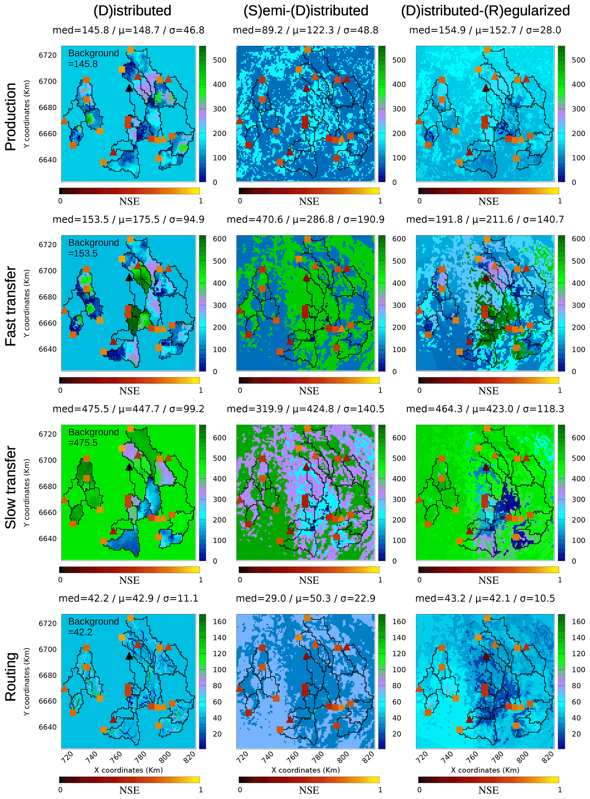
Figure 5 Optimal model parameters for the North study area and for period P1: parameter maps for the distributed, semi-distributed and distributed-regularized calibrations are plotted, while the first guess values from the uniform calibration is specified on the distributed calibration graphics (corresponding to the parameter value outside of the calibration catchments for that calibration experiment). The median, mean and standard deviation values are specified for each parameter map. Squares and triangles represent the NSE score for high flow conditions obtained on the calibration period P1 for the calibration and validation gauges respectively.

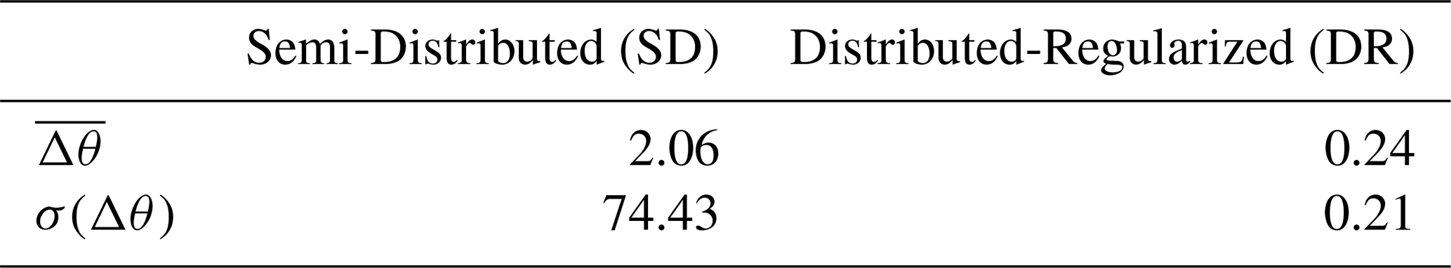
To globally analyse the differences between inferred parameter sets θ_SD and θ_DR obtained for periods P1 and P2 and catchment sets North and South, the relative difference to the uniform first guess θ_U is introduced: $\mathrm{\Delta }{\mathit{\theta }}_{\mathrm{SD}}^{{\mathrm{\Omega }}_k,p,z}=\left|({\widehat{\mathit{\theta }}}_{\mathrm{SD}}^{{\mathrm{\Omega }}_k,p,z}-{{\mathit{\theta }}^{*}}_{\mathrm{U}})\right|/{{\mathit{\theta }}^{*}}_{\mathrm{U}}$ and $\mathrm{\Delta }{\mathit{\theta }}_{\mathrm{DR}}^{{\mathrm{\Omega }}_k,p,z}=\left|({\widehat{\mathit{\theta }}}_{\mathrm{DR}}^{{\mathrm{\Omega }}_k,p,z}-{{\mathit{\theta }}^{*}}_{\mathrm{U}})\right|/{{\mathit{\theta }}^{*}}_{\mathrm{U}}$; where ${\widehat{\mathit{\theta }}}_{\mathrm{SD}}^{{\mathrm{\Omega }}_k,p,z}$ and ${\widehat{\mathit{\theta }}}_{\mathrm{DR}}^{{\mathrm{\Omega }}_k,p,z}$ denote the inferred parameters for each spatial partitioning ${\mathrm{\Omega }}_k=\mathit{\{}{\mathrm{\Omega }}_{\mathrm{1}},\mathrm{\dots },{\mathrm{\Omega }}_{N_k}\mathit{\}}$, period p={P1, P2} and study zone z={North, South}, for the semi-distributed (SD) and distributed-regularized (DR) experiments. The corresponding global spatial averages over each zone, $\stackrel{\mathrm{‾}}{\mathrm{\Delta }{\mathit{\theta }}_{\mathrm{SD}}}$ and $\stackrel{\mathrm{‾}}{\mathrm{\Delta }{\mathit{\theta }}_{\mathrm{DR}}}$, and spatial variances, σ(Δθ_SD) and σ(Δθ_DR), are then computed (see Table 2). The comparison of the averaged relative differences $\stackrel{\mathrm{‾}}{\mathrm{\Delta }{\mathit{\theta }}_{\mathrm{SD}}}>\stackrel{\mathrm{‾}}{\mathrm{\Delta }{\mathit{\theta }}_{\mathrm{DR}}}$ (being equal to 2.06 and 0.24) indicate that the inferred SD parameter set ${\widehat{\mathit{\theta }}}_{\mathrm{SD}}$ strongly deviates from the first guess while the DR ${\widehat{\mathit{\theta }}}_{\mathrm{DR}}$ parameters with physiographic reguarization stay much closer. The comparison of the spatial variances σΔθ_SD>σΔθ_DR (being equal to 74.43 and 0.21) indicates a much higher variablility for the semi-distributed calibration. These results can be seen in terms of deviation from the first guess and spatial variability of the inferred parameters on Fig. 3. The parameter sets from the semi-distributed calibration experiment (SD) are the most variable within the parameter bounds (i.e. higher σ values for the SD parameter maps). The resulting average and median values diverge from the first guess value. The variances of the parameters estimated on the overall domain are also higher in average.

Table 2 Average $\stackrel{\mathrm{‾}}{\mathrm{\Delta }\mathit{\theta }}$ and variance σ(Δθ) values of the relative differences of the optimized model parameter set to the uniform first guess θ_U, for the calibration experiments SD and DR.

When the parameter optimization targets multiple disjoint catchments, the uniform and semi-distributed calibration problems are under-parameterized. This could lead to unexpected optimal parameter sets when catchments exhibit different types of hydrological behavior. This issue occurred in the Southern study area, where the optimal first guess (${\mathit{\theta }}_{\mathrm{U}}=\stackrel{\mathrm{‾}}{\mathit{\theta }}$ being spatially uniform) for the slow transfer reservoir c_tl is equal to 2793 mm for P2 and to 281 mm for P1. For period P2, the semi-distributed calibration (SD) led to an average parameter value $\stackrel{\mathrm{‾}}{c_{\mathrm{tl}}}$ equal to 283 mm; for the distributed calibration, the optimal parameter $\stackrel{\mathrm{‾}}{c_{\mathrm{tl}}}$ could be lower than 500 mm for one catchment and larger than 3000 mm for two others. The uniform and semi-distributed optimization could be driven globally by the performances reached at only one or a few catchments, whereas data quality issues and/or model deficiencies could cause a performance loss for these catchments. Interestingly, the distributed calibration with physiographic regularization (DR) leads to spatially smoother inferred parameter fields.

5 Conclusions

This contribution presented a novel method to regionally calibrate the parameters of a distributed hydrological model using a variational algorithm. This methods relies on classified physiographic map(s) to impose spatial patterns to the parameters, either strongly (SD) via the definition of the control vector or weakly (D) via a regularization term added to the objective function. Both calibration strategies led to similar performances in spatio-temporal validation whereas the distributed-regularized method improved the efficiency scores for the calibration catchments. Both strategies have their own strengths and weaknesses.

The (SD) strategy is the easiest approach to drastically reduce the size of the control vector. However, like the uniform calibration, it is very sensitive to the multi-site optimization function and local model deficiencies and data errors could potentially impact the calibration over the whole area. Moreover, this strategy is very dependent on the choice of the spatial partitioning (i.e, the physiographic descriptors and their number of classes), which should be further explored. It could be interesting to test a combination of these strategies, using the output of the (SD) method as a first guess for the (DR) approach. Finally as the (SD) calibration works similarly to a special case of the MPR approach, we plan to extend this work via the more flexible MPR framework. The fully distributed calibration approach using the physiographic regularization strategy (DR case) showed promising results since: (1) it maximises the model performances at the control stations (MPP similar to the fully distributed approach without regularization); (2) it gives an estimate of the parameters values for the overall area, thus for any ungauged catchments. These regional parameter estimates help to improve the discharge predictions at the pseudo-ungauged validation catchments (which were not used for calibration). One drawback could be the huge size of the control vector. However, the variational optimization using the adjoint model is an efficient method to optimize the parameter vector and the equifinality does not exclusively stem from its size (Jay-Allemand et al., 2020). In our opinion, the distributed-regularized approach is therefore more flexible and adequate for calibrating the parameters of a distributed hydrological model than the (SD) method. We believe that the regularization term can be further enhanced.

The spatio-temporal robustness of the calibrated parameters for (SD) and (DR) approach, is still to be improved: parameter maps are very different between the two calibration subperiods and the MPP at the validation stations are relatively poor compared to the MPP for the calibration stations. This lack of robustness has several causes. First the conceptual model includes parameters with limited physical meaning. Secondly, the optimization problem is overparameterized for the (DR) approach and the first guess values, which play a key role during the optimization, have to be improved using physical priors for example. Last, the lower calibration performance at validation catchments indicates a need to improve the model structure versatility to better adapt to different hydrologic behaviors.

Planned future work will focus on testing other regularizations with a physiographic distance metric and introducing hydrological units, as well as testing the forward model of upscaling and regionalization transfer functions of the MPR approach to upgrade the (SD) strategy. Moreover, a sensivity analysis during the first decisive iterations of the LBFGS-B descent could provide valuable information about the calibration process and its driving components. Finally, a statistical and spatial analysis of the optimized parameters should be performed to search for relations between model parameters and physiographic descriptors and select the most adequate descriptors.