the Creative Commons Attribution 4.0 License.
the Creative Commons Attribution 4.0 License.
 | 18 Apr 2024
Developing Non-Stationary Frequency Relationships for Greater Pamba River basin, Kerala India incorporating dominant climatic precursors
Arathy Nair
Meera Geetha Mohan
Sreedevi Vijayalakshmi
Global climate changes significantly contribute to increased frequency of hydrologic extremes. This significantly underestimates the hydrologic design parameters, bringing of hydro systems to increased failure risk. In order to address this concern, the current practice of development of hydrologic frequency tools need to be updated accounting for non-stationarity. This study first considered a diverse set of statistical tests to examine the trend, change points, non-stationarity and randomness of streamflow, rainfall and temperature time series of scales ranging from daily to annual. The annual maxima time series indicated non stationarity against the stationary behaviour of daily series of hydro-meteorological datasets of the basin. Subsequently, this study developed the Temperature Duration Frequency (TDF), Rainfall Intensity Duration Frequency (IDF) and Flood Frequency (FF) curves of Greater Pamba river basin in Kerala India, the part of which was most severely affected by the near century return period flood event of 2018. The analysis was performed for a multitude of combinations of variations in distribution parameters with time and climatic drivers as physical covariates in the extreme value formulations. The study proposed a novel wavelet coherence (WC) based driver selection of most dominant combination of climatic precursors in developing FF and IDF relations of three locations of Kalloopara, Malakkara and Thumpamon and TDF curve of Kuttanad region in the basin, considering data of 1985–2015 period. The proposed WC framework considers bi-multi-and partial effects of climatic oscillations (COs) like El Niño Southern Oscillation (ENSO), Indian Ocean Dipole (IOD), Pacific Decadal Oscillation (PDO) and North Atlantic Oscillation (NAO) in identifying potential drivers. The different WC formulations captured in-phase relationships of streamflows and rainfall with COs at intra-annual, annual and inter annual scales up to 4 years. The methods showed that addition of climatic precursors improved the NS estimates of flood and rainfall quantiles by more accurately capturing the magnitudes of extreme streamflows and rainfalls of 2018, 2021 than the time covariate formulations. However, the role of COs on extreme temperature is not found to be influential in developing TDF relationships, which needs further investigation.
- Article
(5029 KB) - Full-text XML
- BibTeX
- EndNote


Streamflow; non-stationarity; wavelet; frequency; climatic oscillation
Unpredictable climate variations result in the occurrence of hydrological extremes like floods, droughts etc prompting the exploration of spatiotemporal variability of future extreme streamflow (SF), rainfall (RF) and temperature (Temp) events. To evaluate the consequences on such extreme events due to the uncertainty of projected climate changes, the study on SF, RF and Temp frequency analysis (FA) is indispensable. The hydrologic design parameters are gravely understated by these extremes, increasing the danger of failure for the hydro systems. Taking into account non-stationarity in the distribution parameters will allow the existing method of developing hydrologic frequency tools to be modified in order to meet this issue. The introduction of covariates such as climatic oscillations (COs) and time into the parameters of distribution, so as to deal with the non-stationarity in the hydro-meteorological variable data set is considered to be a widely used technique (Katz et al., 2002; Khaliq et al., 2006; Adlouni et al., 2007). Applications for a wide variety of hydro-climatic extremes, including RF (Ouarda et al., 2019), floods (Villarini et al., 2009), and air temperatures (Ouarda and Charron, 2018), has already been established using this approach.
The wavelet analysis methods are gaining much acceptance while dealing with the analysis of highly irregular, complex, and intermittent non-stationary (NS) time series. For capturing the dominating periodicity and multiscale relationship between two time series, the continuous wavelet transform and bivariate wavelet coherence (BWC) analysis are frequently utilised (Torrence and Compo, 1998; Grinsted et al., 2004). Hu and Si (2016) proposed the multiple wavelet coherence (MWC) approach as an extension of BWC. Mihanovic et al. (2009) introduced the concept of partial wavelet coherence (PWC), thereby evaluating the stand-alone dependence of two variables via a statistical way, after eliminating the effect of other likely governing variables. The concept of wavelet coherence is applied in this study for estimating the teleconnections between different COs and hydro-meteorological variables resulting in the identification of prevalent climatic precursors which can be employed as covariates in the distribution parameters for the development of NS models for non-stationary frequency analysis (NSFA).
India is a country with an extensive river network and SF is considered as the major source of water supply for irrigation and industrial purposes. It is crucial to understand the RF and SF dynamics along with Temp variations to quantify the influence of global climatic drivers at basin scale for improved decision-making. It is well understood that a diverse set of Climatic drivers are influencing the hydro-climatic process of India (Adarsh and Janga Reddy, 2016). Kerala meteorological subdivision of southern India is becoming climatically sensitive in the recent past and the signatures of the same are evident in the form of extreme floods (Anandalekshmi et al., 2019). This study aims to conduct the FA of SF, RF, Temp extremes of Greater Pamba river basin (GPRB), Kerala, India, which is one of the most affected regions in the extreme rare Kerala flood event of 2018, with covariate dependent distribution functions to characterize these extreme events in a NS framework. This study aims (i) to propose a wavelet-based framework for identification of dominant covariate in NS frequency formulations; (ii) to develop NS Intensity-Duration-Frequency (IDF) curves, Flood Frequency (FF) curves and Temperature-Duration-Frequency (TDF) for GPRB, incorporating the dominant climatic precursors obtained from proposed WC framework.
The Greater Pamba river basin consists of rivers Pampa, Manimala and Achencovil rivers flowing through Kerala encompassing the districts of Pathanamthitta, Alappuzha and Kottayam. The three basins of Achenkovil (1484 km2), Pamba (2235 km2) and Manimala (847 km2) together form the GPRB with total drainage area of 4566 km2 and it is classified as a medium-sized basin. The distinct characteristics of three different basins comprised within the GPRB highlight the need for conducting NSFA for the same hydro-meteorological variable recorded in multiple stations. Three SF stations, seven RF stations and one Temp station are considered for the study. The daily SF data for SF1-Kalloopara, SF2-Malakkara and SF3-Thumpamon stations were obtained from India Water Resource Information System (IWRIS) (https://indiawris.gov.in/wris, last access: 3 February 2021). The daily RF and Temp data were gathered from India Meteorological Department (IMD) at a high-resolution of 0.25° × 0.25° (Pai et al., 2014) and 1° × 1° (Srivastava et al., 2009) gridded data set respectively. All the datasets were collected for a span of 31 years (1985–2015). In case of NSFA, the daily SF data was converted to annual maximum SF for the development of FF curves. While the daily RF data was used to extract annual maximum series for 10 durations (1, 3, 6, 12, 18, 24, 36, 48, 60, 72 h) to develop IDF curves and the daily maximum Temp data was extracted to annual maximum Temp over 6 durations (1, 2, 4, 6, 8, 10 d) for developing TDF curves. The locations of the hydro-meteorological stations and grid points are indicated in Fig. 1. Four large-scale COs namely, El Niño Southern Oscillation (ENSO), North Atlantic Oscillation (NAO), Pacific Decadal Oscillation (PDO) and Indian Ocean Dipole (IOD) are considered as potential drivers for teleconnection analysis (Krishnamurthy and Goswami, 2000; Krishnan and Sugi, 2003; Mokhov et al., 2012; Li and Chen, 2014; Azad and Rajeevan, 2016; Rathinasamy et al., 2019; Yeditha et al., 2022). The climatic indices are taken from https://psl.noaa.gov/gcos_wgsp/Timeseries/ (last access: 3 February 2021) for the period 1985 to 2015.

Figure 1Location of hydro-meteorological stations and grid points in GPRB, Kerala, India.
3.1 Statistical analysis
A number of statistical tests are used to analyse the temporal variance in the SF, RF, and Temp time series. The study of descriptive statistical analysis includes looking at concepts like trend, stationarity, change point, and randomness. Trend in the timeseries is estimated using MK test (Mann, 1945; Kendall, 1975) and Sen's slope test (Sen, 1968). The trend analysis shows general trend in a time series, but the stationarity test shows how the mean and variance vary with time. The Augmented Dickey-Fuller (ADF) (Dickey and Fuller, 1979) and KPSS test (Kwiatkowski et al., 1992) are used for testing stationarity of different time series, at 5 % significance. The significant homogeneous and non-homogeneous nature of the times series was tested by Pettit's change point test (Pettit, 1979), Standard Normal Homogeneity test (Alexandersson and Moberg, 1997) and Buishand range test (Buishand et al., 2008). Randomness of the chosen variable time series of each station were tested using Runs test.

3.2 Wavelet Coherence analysis
A wavelet is defined as a small wave which has good ability in representing a signal locally in both time and frequency domains. The fundamental principle of wavelet transforms (WT) is to decompose the time series into its wavelets which are scaled and translated version of the mother wavelet (Torrence and Compo, 1998; Grinsted et al., 2004). The key benefit of using WT is that it reveals the hidden non-stationarity information in the original variable. The continuous wavelet transform (CWT) has been widely used for hydro-climatic teleconnection studies, while discrete wavelet transform (DWT) is popular for hydrological forecasting (Sang, 2013; Nourani et al., 2014). While CWT work on all the scales to analyse time series but the coherence will be significant only at certain time scale and their strength also differ with time scale. Considering the benefits of WT, methods like cross-wavelet analysis (XWT) and wavelet coherence (WC) have also become effective instruments for examining potential connections between two signals (Grinsted et al., 2004). XWT identifies only the regions with a high common power in the two-time series and WC measures how coherent XWT is in the time-frequency domain.
BWC quantifies the relationship between two variables, i.e., one hydro-meteorological variable and one CO. MWC is important to assess the simultaneous influence of more than one teleconnection at various timescales. Apart from this, PWC is accomplished to determine the standalone relationship between a CO and hydro-meteorological variable. For instance, two COs, ENSO and IOD, which are both highly connected, may have an impact on streamflow (SF2). In this case, WC analysis of the link between SF2 and IOD automatically takes ENSO's impact into account. This could lead to a misinterpretation of the true connection between SF2 and IOD. Hence solitary impact of each CO on hydro-meteorological variable must therefore be investigated using PWC.
In the case of teleconnection investigations, it is desirable to examine the relationship between two time series (hydro-meteorological variable and CO) in the time-frequency domain. However, the use of all scales results in redundant data, which significantly raises the cost of calculation and lowers the model's performance. In this study, application is for identifying the dominant driver using wavelet analysis, for which, quantifying the strength is essential. Therefore, the relative dominance of single or multiple COs on the hydro-meteorological variable is measured using the Average Wavelet Coherence (AWC) and the Percentage of Significant Coherence (PoSC) (Song et al., 2020; Sreedevi et al., 2022). By averaging the WC generated across all dominant scales using the obtained coherence values, the AWC may be determined. The PoSC can be calculated by dividing the total number of power values created in the WC computation by the number of significant power values. Greater dominance is indicated by higher PoSC and AWC scores. Even though the coherence between COs and hydro-meteorological variables may grow with the addition of more COs, an increase in the PoSC value of at least 5 % must be seen in order to draw the conclusion that the new addition has any practical impact.
3.3 Development of S and NS models
The Cumulative Distribution Function (CDF) of Generalized Extreme Value (GEV) distribution used for developing FF, IDF and TDF relationship is
Where,
Where μ= location parameter, σ= scale parameter and ξ= shape parameter.
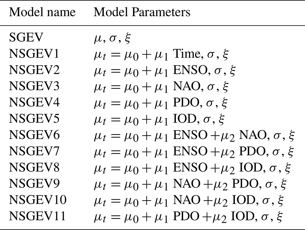
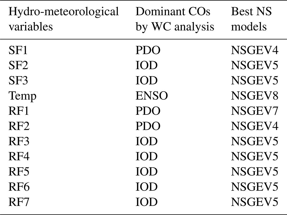
In the NS case, the distribution parameters namely location and scale parameters are made dependent on covariates which can represent a CO or time. The shape parameter of the GEV is kept as a constant. The COs required for developing NS models were chosen based on the dominant COs obtained from the WC analysis. Table 1 indicates the best NS models used in this study. The method of Maximum Likelihood estimation (MLE) (Khaliq et al., 2006) is used for parameter estimation and the best fit model is identified with the help of Akaike Information Criterion (AIC) (Akaike, 1974). The model resulting in smallest AIC value is considered to be the best performing model.
The NS return levels for various return periods, RPs (T in years) are computed using Eq. (2). In the case of NS models, 95 percentiles of the covariate dependent parameters from the past observations are taken as a representative value for the location and scale parameters.
4.1 Statistical analysis
The mean, standard deviation, skewness, kurtosis, minimum and maximum values of the chosen SF, RF and Temp stations belonging to GPRB was computed. All the datasets are positively skewed to the right with high skewness except for Temp data set which is slightly skewed. In terms of kurtosis, all the data sets have a leptokurtic distribution (k>3; sharply peaked with heavy tails) while Temp data set have a platykurtic distribution (k∼0; flat peak and has more dispersed values with lighter tails). Sen's slope test was used to evaluate the size of the change while the MK test was used to determine the significance of the trend. All the RF grid points and SF1 station was found to have an increasing trend, while Temp and SF2, SF3 stations followed a decreasing trend. According to ADF test, SF1, RF4 and RF5 were found to be stationary while others were non-stationary whereas in the case of KPSS test, all the stations except for RF6 and RF7 were found to be stationary. The results of the change point analysis pointed to a considerable sudden change at each location. All the data sets were proved to be non-random in nature of occurrence with the help of Runs test. The overall results of the statistical analysis pave way to the presence of trend, non-stationarity, inhomogeneity and non-randomness in the SF, RF and Temp data sets.
4.2 Wavelet Coherence analysis
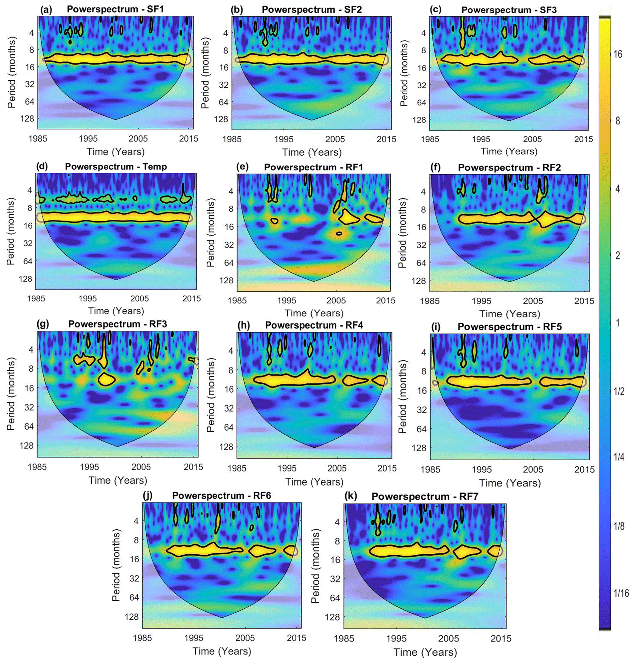
The WC analysis observed annual periodicity (8–16 months) for most of the time series for all stations, except for RF1 and RF3. Lower periodicities (2, 4 and 6 months) are observed mainly for Temp station, but there is localized presence in various time domain for the same periodicities for SF and RF stations as well. A pictorial representation of the same is given in Fig. 2. The results of BWC analysis of SF2 (Malakkara) station with the COs are presented in Fig. 3 along with two samples of MWC as well.
Due to space constraints, the BWC, PWC and MWC results obtained for one sample station; SF2 (Malakkara) station is only discussed in detail. BWC analysis for SF2-ENSO and SF2-NAO doesn't show any significant periodicity, however some localized contours were found around the periodicity of 2–48 months. For SF2-IOD across the time periods of 1990–2003, 2005–2007, and 2011–2014, the coherence correlations predominately range between periodicities of 8–16 months. In the case of SF2-PDO inter-decadal ranges were observed for the period 1988–1998 with a periodicity of 32–64 months. Higher AWC and PoSC values were obtained for SF2-IOD (AWC = 0.478 and PoSC = 25.03). The combined influence of PDO and IOD produced the highest coherence values for SF2 station for MWC-two factor analysis (AWC = 0.75, PoSC = 41.71). Among the three-factor scenarios, the ENSO, PDO and IOD combination produced the highest coherence score. On considering all the COs, the coherence value was at its maximum (AWC = 0.93, PoSC = 48.03).
All of the PWC's AWC and PoSC values were lower than the BWC readings. The maximum reduction in PoSC value resulted in ENSO (from 23.36 %) after the removal of NAO (to 5.44 %) and PDO (to 7.32 %) from it. The removal of IOD had very less effect on ENSO. The influence of PDO on SF2 station is highly influenced by ENSO, NAO and IOD. PWC results of IOD and NAO showed less reduction in PoSC values which also indicates that IOD and NAO are not being strongly modulated by other COs. Similarly bi-multi-and partial effects of COs on all the other hydro-meteorological variables were evaluated. IOD, PDO, ENSO and its combinations were found to be more influential for all the hydro-meteorological variables in general.
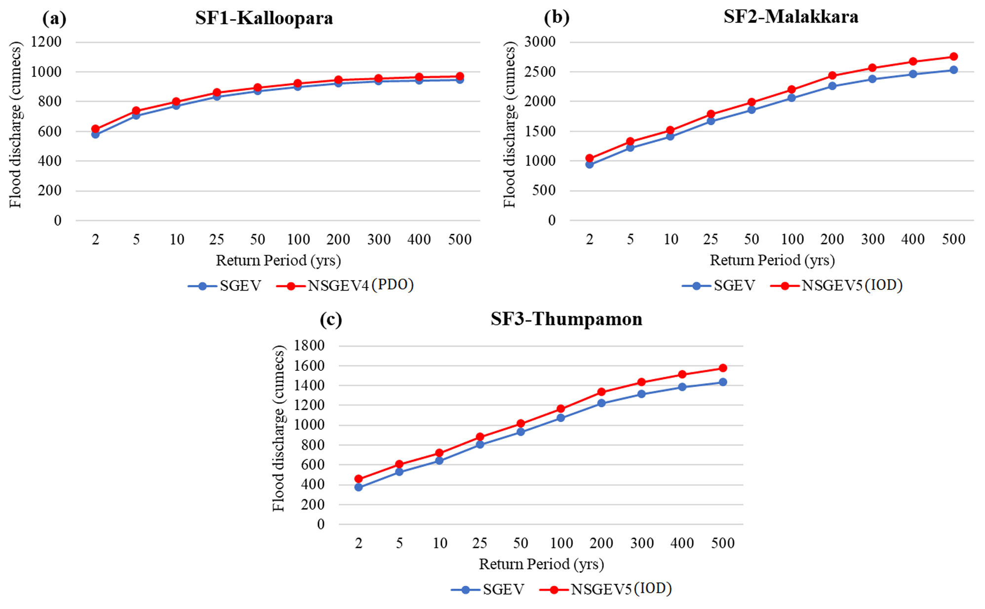
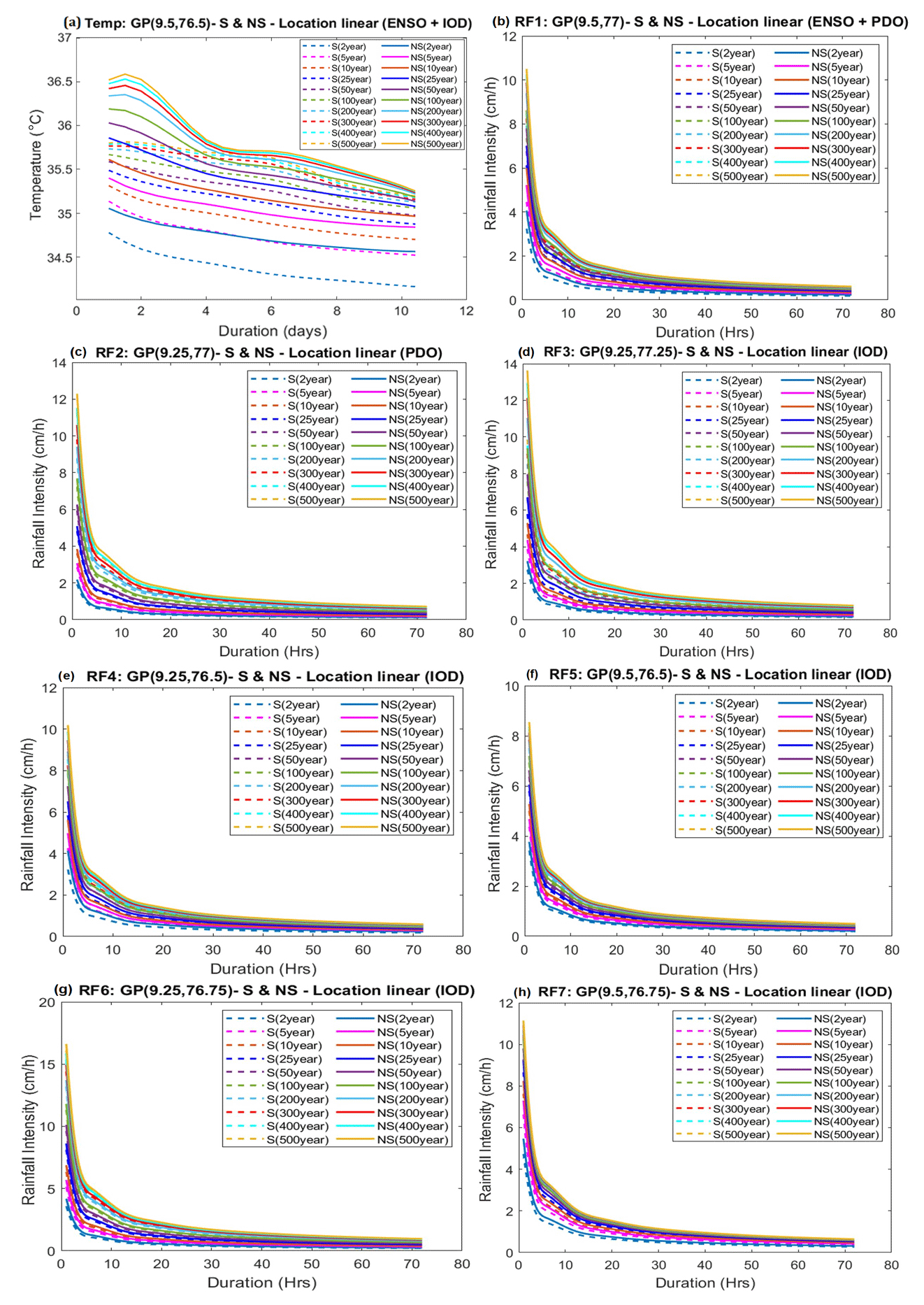
Table 2Comparison of dominant COs by WC analysis and best NS models.
4.3 Stationary and Non-Stationary models
The S and NS analysis was carried out for all the hydro-meteorological variables by developing GEV models as mentioned in Sect. 3.3 using all possible combinations of Time and CO as covariate and the best fit model was identified with the help of AIC values (Table 2). The FF, IDF and TDF curves developed for corresponding stations based on the best fit NS model is given in Figs. 4 and 5. It can be seen that all the best fit NS models were based on CO formulations. Additionally, it should be highlighted that the CO, which showed a strong teleconnection with the hydro-meteorological variable in relation to AWC and PoSC values, emerged as the best covariate that addresses the non-stationarities in terms of climate-induced NS model for FF, IDF and TDF analyses. For instance, the best NS model obtained for SF2-Malakkara station is location parameter linearly varying with IOD as covariate and it can be clearly seen that the most dominant CO for SF2 station is IOD as per AWC and PoSC values of WC analysis as discussed in Sect. 4.2. The same was applicable for all the hydro-meteorological stations. The findings, which are summarised in Table 2, support the conclusion that the dominating COs derived from the WC analysis turned out to be the best covariate to describe NS behaviour of the respective hydro-meteorological stations. As a result of this study, it can be inferred that using a wavelet-based framework to identify dominant covariates will significantly help in determining the best covariate to describe each station's non-stationary behaviour. Also, teleconnection investigations over various frequency-time scales using BWC, MWC and PWC helped in the identification of key temporal features or events in a signal, such as discontinuities, rapid leaps and shifts, and patterns of dominant variability over the chosen time period.
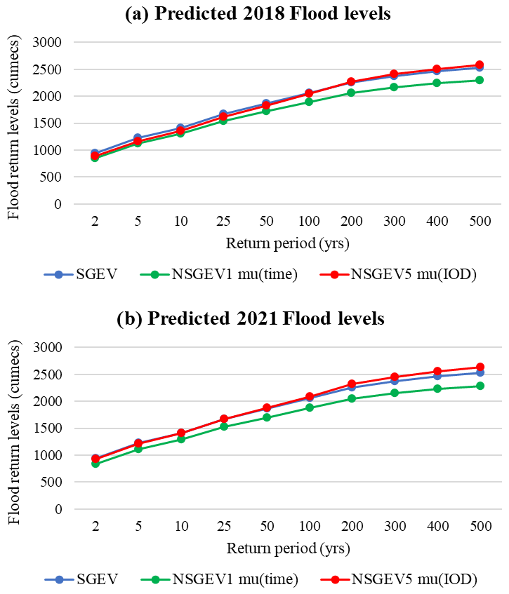
The physical connections between the covariates and the local hydrology of GPRB was also examined to validate our findings. For instance, Maximum flood discharge of the basin (1988 cumecs) was recorded in the year 1994, a year with a predominately positive IOD event (Kumar et al., 2019). Also, the peak annual maximum temperature was observed in the year 1997, where the combined effect of ENSO and IOD was significantly predominant (Kumar et al., 2019). The results obtained using the best-fitting NS model, NSGEV8, for the Temp grid point, where the location parameter varies linearly with ENSO and IOD, validates the same. Hence, it can be concluded that the annual maximum value of the hydro-meteorological variable peaked in the year where their respective best fit CO (Tables 1 and 2) effect was predominant. Additionally, the SF, RF and Temp return levels for various RPs were predicted using S and NS model with time and COs as covariates. A sample of 2018 and 2021 floods predicted for SF2 station using all the three models is shown in Fig. 6. According to the Central Water Commission's (CWC) “Report on Kerala Flood and Solutions” from 2018, the return period of the 2018 Kerala flood was unquestionably greater than 100 years, leading to the conclusion that the addition of climatic precursors improved the prediction of NS estimates of the SF and RF quantiles when compared to S and time covariate formulations (Fig. 6), but that this was not the case for the temperature return level, which requires further research.
This study proposed a novel framework in developing NS models based on the identification of best covariates using WC analysis, based on the assumption that the non-stationarity of the signal is well explained by the CO. It is worth noting that the model complexity increases while trying to incorporate non-stationarities related to climate change and variability. Hence, it is quite evident that model uncertainty will also increase as the complexity increases. Uncertainty analysis of NS models is an area which requires further exploration and future works are needed to access the uncertainty at covariate and parameter scale for developing reliable NS models.
The hydro-meteorological variables namely, three SF, one Temp and seven RF stations belonging to GPRB were found to have significant trend, non-stationarity, inhomogeneity and non-randomness in the dataset. The main focus of the study is to develop FF, IDF and TDF relationships in a NS framework by incorporating COs and Time as covariates in the distribution parameters. Out of the four chosen COs, the most dominant climatic precursors were identified using WC analysis. A multitude of combinations of COs with the hydro-meteorological variables were analysed via CWT, BWC, MWC and PWC. According to AWC and PoSC values of wavelet coherence analysis, it is discovered that IOD has a major impact on the basin scale hydrology. The creation of the NS model for FA was greatly aided by the covariate selection made using the WC based driver selection of the most dominating combination of climatic precursors. It was found that NS models where location parameter is varying in correspondence with IDO, PDO, ENSO and its combinations turned out to be the best fit models for the respective stations. In-phase correlations of SF and RF with COs at intra-annual, annual, and inter-annual periods up to 4 years were captured by several WC formulations. The NS flood and RF return level estimates were better with the addition of climatic antecedents than with the time covariate formulations. The same was verified by precisely simulating the severe SF and RF magnitudes of 2018 and 2021 utilising CO as a covariate in NS models.
All the data used for this work are freely available and the resource agency which provides the same are mentioned in Sect. 2 (Gridded rainfall data – Pai et al., 2014; Gridded temperature data – Srivastava et al., 2009; Streamflow data – https://indiawris.gov.in/wris, last access: 3 February 2021, India-WRIS, 2021; Climatic indices data – https://psl.noaa.gov/gcos_wgsp/Timeseries/, last access: 3 February 2021, GCOS, 2020). The software codes used in the study are developed by the authors. The current work is a part of the funded project sanctioned by Science Engineering and Research Board, Department of Science and Technology (DST-SERB) India. The project work is still under progress; hence the codes cannot be made available in public. However, under genuine and reasonable requests, the codes will be made available by the corresponding author.
AS, AN and MGM conceptualized the idea. AN, MGM and SV done the formal analysis and plotting, AN and MGM drafted the manuscript, AS supervised and revised the manuscript. All authors reviewed the manuscript.
The contact author has declared that none of the authors has any competing interests.
Publisher's note: Copernicus Publications remains neutral with regard to jurisdictional claims in published maps and institutional affiliations.
This article is part of the special issue “IAHS2022 – Hydrological sciences in the Anthropocene: Variability and change across space, time, extremes, and interfaces”. It is a result of the XIth Scientific Assembly of the International Association of Hydrological Sciences (IAHS 2022), Montpellier, France, 29 May–3 June 2022.
The authors acknowledge DST-SERB, India for sanctioning the project entitled “Developing Non-Stationary Frequency Relationships of Hydro-climatic Extremes of Kerala Meteorological Subdivision under Changing Climate Scenario”, (File Number: CRG/2021/003688) for which the present work will function as a component. We would like to thank India-WRIS for giving access to daily streamflow data, IMD for providing gridded daily maximum temperature and rainfall data and also GCOS for supplying climate indices data for the years 1985–2015. Authors thank IAHS for supporting the corresponding author with SYSTA to present the work in the 11th IAHS Scientific Assembly held at Montpellier France during 29 May–3 June 2022.
This paper was edited by Christophe Cudennec and reviewed by two anonymous referees.
Adarsh, S. and Janga Reddy, M.: Analysing the hydroclimatic teleconnections of summer monsoon rainfall in Kerala, India using Multivariate Empirical Mode Decomposition and time dependent intrinsic Correlation, IEEE Geosci. Remote Sens. Lett. 13, 1221–1225, 2016.
Adlouni, S. E., Ouarda, T. B. M. J., Zhang, X., Roy, R., and Bobée, B.: Generalized maximum likelihood estimators for the nonstationary generalized extreme value model, Water Resour. Res., 43, W03410, https://doi.org/10.1029/2005WR004545, 2007.
Akaike, H.: A new look at the statistical model identification, IEEE T. Automatic Control, 19, 716–23, 1974.
Alexandersson, H. and Moberg, A.: Homogenization of Swedish Temperature data. Part I: homogeneity test for linear trends, Int. J. Climatol., 17, 25–34, 1997.
Anandalekshmi, A., Panicker, S. T., Adarsh, S., Siddik, M. A., Aloysius, S., and Mehjabin, M.: Modeling the concurrent impact of extreme rainfall and reservoir storage on Kerala Floods 2018: A Copula approach, Model. Earth Syst. Environ., 5, 1283–1296, 2019.
Azad, S. and Rajeevan, M.: Possible shift in the ENSO-Indian monsoon rainfall relationship under future global warming, Sci. Rep.-UK, 6, 20145, https://doi.org/10.1038/srep20145, 2016.
Buishand, T. A., de Haan, L., and Zhou, C.: On spatial extremes: with application to a rainfall problem, Ann. Appl. Stat., 2, 624–642, 2008.
Dickey, D. A. and Fuller, W. A.: Distribution of the estimators for autoregressive time series with a unit root, J. Am. Stat. Assoc., 74, 427–431, 1979.
GCOS: Download Climate Timeseries, GCOS [data set], https://psl.noaa.gov/gcos_wgsp/Timeseries/ (last access: 3 February 2021), 2020.
Grinsted, A., Moore, J. C., and Jevrejeva, S.: Application of the cross wavelet transform and wavelet coherence to geophysical time series, Nonlin. Processes Geophys., 11, 561–566, https://doi.org/10.5194/npg-11-561-2004, 2004.
Hu, W. and Si, B. C.: Technical note: Multiple wavelet coherence for untangling scale-specific and localized multivariate relationships in geosciences, Hydrol. Earth Syst. Sci., 20, 3183–3191, https://doi.org/10.5194/hess-20-3183-2016, 2016.
India-WRIS: India Water Resources Information System, India-WRIS [data set], https://indiawris.gov.in/wris, last access: 3 February 2021.
Katz, R. W., Parlang, M. B., and Naveau, P.: Statistics of extremes in hydrology, Adv. Water Resour., 25, 1287–1304, 2002.
Kendall, M. G.: Rank Correlation Methods, 4th edn., Charles Griffin, London, 1975.
Khaliq, M. N., Ouarda, T. B. M. J., Ondo, J. C., Gachon, P., and Bobée, B.: Frequency analysis of a sequence of dependent and/or non-stationary hydro-meteorological observations: a review, J. Hydrol., 329, 534–552, 2006.
Krishnamurthy, V. and Goswami, B. N.: Indian Mon soon–ENSO Relationship on Interdecadal Timescale, J. Climate, 13, 579–595, 2000.
Krishnan, R. and Sugi, M.: Pacific decadal oscillation and variability of the Indian summer monsoon rainfall, Clim. Dynam., 21, 233–242, 2003.
Kumar, P., Kaur, S., Weller, E., and Min, S. K.: Influence of natural climate variability on the extreme ocean surface wave heights over the Indian Ocean, J. Geophys. Res.-Oceans, 124, 6176–6199, https://doi.org/10.1029/2019JC015391, 2019.
Kwiatkowski, D., Phillips, P. C. B., Schmidt, P., and Shin, Y.: Testing the null hypothesis of stationarity against the alternative of a unit root how sure are we that economic time series have a unit root?, J. Econ., 54, 159–178, 1992.
Li, Q. and Chen, J.: Teleconnection between ENSO and climate in South China, Stoch. Environ. Res. Risk. Assess., 28, 927–941, 2014.
Mann, H. B.: Non-parametric tests against trend, Econometrica, 13, 163–171, 1945.
Mihanovic, H., Orlic, M., and Pasaric, Z.: Diurnal thermocline oscillations driven by tidal flow around an island in the Middle Adriatic, J. Marine Syst., 78, S157–S168, 2009.
Mokhov, II., Smirnov, D. A., Nakonechny, P. I., Kozlenko, S. S., and Kurths, J.: Relationship between El-Ninño/Southern oscillation and the Indian monsoon, Izv. Atmos. Ocean Phys., 48, 47–56, https://doi.org/10.1134/S0001433812010082, 2012.
Nourani, V., Hosseini Baghanam, A., Adamowski, J., and Kisi, O.: Applications of hybrid wavelet – Artificial Intelligence models in hydrology: A review, J. Hydrol., 514, 358–377, 2014.
Ouarda, T. B. M. J. and Charron, C.: Nonstationary Temperature-duration-frequency curves, Sci. Rep., 8, 15493, https://doi.org/10.1038/s41598-018-33974-y., 2018.
Ouarda, T. B. M. J., Yousef, L. A., and Charron, C.: Non-stationary intensity–duration-frequency curves integrating information concerning teleconnections and climate change, Int. J. Climatol., 39, 2306–2323, 2019.
Pai, D. S., Latha, S., Rajeevan, M., Sreejith, O. P., Satbhai, N. S., and Mukhopadhyay, B.: Development of a new high spatial resolution (0.25° × 0.25°) Long period (1901–2010) daily gridded rainfall data set over India and its comparison with existing data sets over the region, MAUSAM, 65, 1–18, https://doi.org/10.54302/mausam.v65i1.851, 2014.
Pettitt, A. N.: A non-parametric approach to the change-point problem, Appl. Stat., 28, 126–135, 1979.
Rathinasamy, M., Agarwal, A., Sivakumar, B., Marwan, N., and Kurths, J.: Wavelet analysis of precipitation extremes over India and teleconnections to climate indices, Stoch. Environ. Res. Risk Assess., 33, 2053–2069, https://doi.org/10.1007/s00477-019-01738-3, 2019.
Sang, Y. F.: A review on the applications of wavelet transform in hydrology time series analysis, Atmos. Res., 122, 8–15, 2013.
Sen, P. K.: Estimates of the regression coefficient based on Kendall's tau, J. Am. Stat. Assoc., 63, 1379–1389, 1968.
Song, X., Zhang, C., Zhang, J., Zou, X., Mo, Y., and Tian, Y.: Potential linkages of precipitation extremes in Beijing-Tianjin-Hebei region, China, with large-scale climate patterns using wavelet-based approaches, Theor. Appl. Climatol., 141, 1251–1269, 2020.
Sreedevi, V., Adarsh, S., and Nourani, V.: Multiscale Coherence Analysis of Reference Evapotranspiration of North Western Iran Using Wavelet Transform, J. Wat Clim. Change, 13, 505–521, 2022.
Srivastava, A. K., Rajeevan, M., and Kshirsagar, S. R.: Development of High Resolution Daily Gridded Temperature Data Set (1969–2005) for the Indian Region, Atmos. Sci. Lett., 10, 249–254, https://doi.org/10.1002/asl.232, 2009.
Torrence, G. and Compo, G. P.: A practical guide to wavelet analysis, B. Am. Meteorol. Soc., 79, 61–78, 1998.
Villarini, G., Smith, J. A., Serinaldi, F., Bales, J., Bates, P. D., Krajewski, W. F.: Flood frequency analysis for nonstationary annual peak records in an urban drainage basin, Adv. Water Resour., 32, 1255–1266, 2009.
Yeditha, P. K., Pant, T., Rathinasamy, M., and Agarwal, A.: Multi-scale investigation on streamflow temporal variability and its connection to global climate indices for unregulated rivers in India, J. Wat. Clim. Change, 13, 735–757, 2022.