Assessment of SMADI and SWDI agricultural drought indices using remotely sensed root zone soil moisture

The increasing frequency of drought events has expanded the research interest in drought monitoring. In this regard, remote sensing is a useful tool to globally mapping the agricultural drought. While this type of drought is directly linked to the availability of root zone soil moisture (RZSM) for plants growth, current satellite soil moisture observations only characterize the water content of the surface soil layer (0–5 cm). In this study, two soil moisture-based agricultural drought indices were obtained at a weekly rate from June 2010 to December 2016, using RZSM estimations at 1 km from the Soil Moisture and Ocean Salinity (SMOS) satellite, instead of surface soil moisture (SSM). The RZSM was estimated by applying the Soil Water Index (SWI) model to the SMOS SSM. The Soil Moisture Agricultural Drought Index (SMADI) and the Soil Water Deficit Index (SWDI) were assessed over the Castilla y León region (Spain) at 1 km spatial resolution. They were compared with the Atmospheric Water Deficit (AWD) and the Crop Moisture Index (CMI), both computed at different weather stations distributed over the study area. The level of agreement was analyzed through statistical correlation. Results showed that the use of RZSM does not influence the characterization of drought, both for SMADI and SWDI.

1 Introduction

In the last years, drought has been one of the natural disasters with the worst impact in the agricultural regions worldwide (FAO, 2018). Traditional drought indices, such as the Palmer Drought Severity Index, PDSI (Palmer, 1965), the Standardized Precipitation Index, SPI (McKee et al., 1993) or the Atmospheric Water Deficit, AWD (Purcell et al., 2003), utilize meteorological variables as drought indicators. However, the agricultural drought begins when the available soil moisture drops below a critical threshold, which can cause crop stress and adversely affect yields (Panu and Sharma, 2002; Mishra and Singh, 2010). Then, the soil moisture can be considered as the key variable of this type of drought.

The most used agricultural drought index is the Crop Moisture Index, CMI (Palmer, 1968). It is usually computed alongside the PDSI from evapotranspiration (ET₀) deficit and moisture excess, using climate-based data. Furthermore, several soil moisture-based agricultural drought indices are being developed, as the Soil Moisture Deficit Index, SMDI (Narasimhan and Srinivasan, 2005), the Soil Water Deficit Index, SWDI (Martínez-Fernández et al., 2015) and the Soil Moisture Agricultural Drought Index, SMADI (Sánchez et al., 2016), among others.

Nowadays, there are two missions specifically dedicated to global measuring soil moisture. The first is the Soil Moisture and Ocean Salinity (SMOS), launched in 2009 by the European Space Agency, ESA (Kerr et al., 2016). SMOS L2 surface soil moisture at 15 km is operationally distributed by ESA. In addition, a downscaled SMOS L4 surface soil moisture at 1 km is provided by the Barcelona Expert Centre (BEC). The second satellite is the Soil Moisture Active Passive (SMAP) of the National Aeronautics and Space Administration (NASA), in orbit since 2015 (Chan et al, 2016). SMAP L2 surface soil moisture maps at 36 and 9 km are disseminated by NASA. These remotely sensed soil moisture observations are only capable of measuring the surface soil moisture (SSM) of the top soil layer (approx. 0–5 cm). Meanwhile, the roots of common crops are enclosed at deeper soil layers, around 0–1 m depth (Allen et al., 1998), where the root zone soil moisture (RZSM) is defined.

The RZSM can be estimated using hydrological or land surface models. Commonly, these models are complex, requiring a high computational processing cost and many input variables as well as data assimilation techniques (Muñoz-Sabater et al., 2007; Das et al., 2010; Dumedah et al., 2015). There are two operational RZSM products based on SMOS and SMAP, the SMOS L4 RZSM at 25 km provided by the Centre d'Etudes Spatiales de la Biosphere, CESBIO (Al Bitar et al., 2013) and the SMAP L4 RZSM at 9 km, provided by the National Snow and Ice Data Center Distributed Active Archive Center, NSIDC DAAC (Reichle et al., 2017). An alternative to these hydrological models is the Soil Water Index, SWI (Wagner et al., 1999; Albergel et al., 2008). The SWI model is an exponential filter that is easy to apply for estimating the RZSM.

Since the soil profile behaves as a filter between incoming water and processes that remove it from the hydrological system (Entekhabi et al., 1996), the SSM can be highly affected by anomalous temperature or precipitation events of a particular day. Under these circumstances, the SSM may reflect inaccurate soil water conditions, whereas the RZSM actually indicates the available water storage for plants growth. Therefore, the RZSM is expected to be more appropriate than the SSM for the agricultural drought monitoring. Nonetheless, a limited number of drought indices have been calculated using in situ RZSM (Hunt et al., 2009; Martínez-Fernández et al., 2015), but few drought studies were found using the RZSM estimated from satellite SSM observations (Tobin et al., 2017).

This work aimed to assess the impact of the remotely sensed RZSM in two soil moisture-based agricultural drought indices, the SMADI and the SWDI, instead of using SSM. Both SMADI and SWDI indices were weekly estimated from June 2010 to December 2016 over the agricultural areas of the Castilla y León region, Spain. To assess the behavior of the indices, they were compared through statistical correlation with AWD and CMI, both obtained from meteorological data acquired at different weather stations distributed over the study area.

2 Study area

This research was developed in the Castilla y León region, located at the northwest of Spain (39.85–43.35^∘ N; 7.35–1.65^∘ W), as study area. This region is mainly characterized by a large plain surrounded by mountains to the North, South and East. The extension of the plain is approxi-mately 65 000 km² and has a mean altitude of 800 m. Its climate is continental semi-arid Mediterranean with a mean annual temperature of 11.8 ^∘C. The Castilla y León region suffers of scarcity of water, with an average annual precipitation of 450 mm (González-Zamora et al., 2015). Despite this, it is one of the largest agricultural areas of the European Union, chiefly dedicated to rainfed agriculture. In this region, croplands are usually located in areas with an elevation lower than 1100 m, while areas at higher altitudes are mainly covered by forest-pasture. The main crop types are cereals (73.5 %), industrial crops (13 %), forages (8 %), and legumes, tubers and vegetables (5.5 %) (Pablos et al., 2017).

3 Data

3.1 In situ data

Three climatic networks were used in this study (Fig. 1). The first is the Soil Moisture Measurement Stations Network of the University of Salamanca, REMEDHUS (González-Zamora et al., 2015). Several weather stations are also installed in REMEDHUS, from which the Villamor station was selected. The second is Inforiego, an agro-meteorological network from the Agriculture Technological Institute of Castilla y León (ITACyL) that is dedicated to irrigation assessment. The third one is the Spanish Meteorological Agency (AEMet) network, which provided long-term weather data.

Figure 1 Digital elevation model (DEM) map of the Castilla y León region showing the location of the REMEDHUS, Inforiego and AEMet stations.

Daily data (precipitation, air temperature, relative humidity, solar radiation and wind speed) measured by the 22 agro-meteorological stations of the Inforiego network and the Villamor station, were used from June 2010 to December 2016. Similarly, historical records from 1985 to 2016 of daily air temperature and precipitation acquired by six stations of the AEMet network were utilized.

As other ancillary data, the digital elevation model (DEM) provided by the ITACYL at 25 m of spatial resolution was used for discriminating the agricultural areas of the study region.

The surface soil database of the Duero basin from the ITACyL was also employed. It contains approximately ten thousand samples with information of soil texture and organic matter (OM) contents.

3.2 SMOS-BEC L4 SSM

The cloud free SMOS-BEC L4 SSM v.3 product at 1 km over the Iberian Peninsula was used from June 2010 to December 2016. These SSM maps are obtained from the combination of daily SMOS brightness temperature and SSM (L1C and L2, both v.620), 16-day Terra Moderate Resolution Imaging Spectroradiometer (MODIS) Normalized Difference Vegetation Index, NDVI (MOD13A2 v.5) and European Centre for Medium-Range Weather Forecasts (ECMWF) land surface temperature (LST) in a downscaling algorithm (Portal et al., 2017). The downscaling is separately applied for ascending and descending SMOS orbits (06:00 and 18:00 local time, respectively).

3.3 SMOS-CESBIO L4 RZSM

The global SMOS-CESBIO L4 RZSM v.300 at a 25 km Equal Area Scalable Earth (EASE)-2 grid was employed. The RZSM maps are obtained through a double soil layer (0–40 and 40–100 cm) hydrological model (Al Bitar et al., 2013). This model is daily applied for ascending and descending orbits, but it is driven by a 3 day average of the SMOS-CESBIO L3 SSM and ancillary datasets, such as the MODIS NDVI and climatic data.

3.4 SMAP L4 SSM and RZSM

The global SMAP L4 SSM and RZSM v.3 geophysical data maps at a 9 km EASE-2 grid were used from 31 March 2015 to December 2016. Both variables (SSM and RZSM) have a temporal resolution of 3 h and are included in the same product. The SSM and RZSM are obtained by means of the NASA Catchment land surface model. This model is driven by the daily SMAP brightness temperature, previously interpolated to 9 km, together with observation-based surface meteorological data forcing, including precipitation (Reichle et al, 2017).

3.5 MODIS reflectance and LST

The day time Aqua MODIS LST at 1 km (MYD11A1 v.6) and surface reflectance (SR) at 500 m (MYD09GA v.6) in red (∼660 nm) and near infrared bands (∼860 nm), provided by the U.S. Land Processes Distributed Active Archive Center (LP DAAC, https://lpdaac.usgs.gov, last access: 7 August 2018), were used from June 2010 to December 2016. The SR data were employed to calculate the NDVI. Both LST and SR are projected to a tile-based sinusoidal grid. The four tiles covering the study area (h17v04, h17v05, h18v04 and h18v05) were selected.

4 Methods

4.1 Data pre-processing

The agricultural drought indices were only computed at the agricultural areas of the Castilla y León region. These areas were delimited by an elevation criterion and soils with OM content higher than 4 % were also discarded, because usually these conditions are out of the agricultural domain under Mediterranean conditions. To do so, the DEM was interpolated from the 25 m grid to a regular 1 km grid to match the final resolution that was used in this work (Fig. 1). Then, all input data were clipped with a mask, keeping data in areas with altitudes lower than 1100 m and discarding the rest.

Regarding the soil database from the ITACyL, surface samples over forested areas, defined as those with OM contents higher than 4 %, were discarded. The remaining samples were interpolated to the same 1 km grid used for the indices to obtain four maps (sand, clay, silt and OM).

The SMOS-BEC L4 SSM maps were firstly resampled to the regular 1 km grid. For each day, the ascending and descending maps were averaged. The resulting daily maps were weekly averaged, because the weekly temporal rate fits better with the agricultural management schedule.

In MODIS data, the 4 tiles with the LST and SR maps were mosaicked and clipped to select the study area. Later, the resulting maps were resampled, at their native spatial resolutions (LST at 1 km and SR at 500 m) from the sinusoidal grid to a regular one. The daily SR maps were masked out using the cloud and snow/ice flags, and filtered at the highest quality. The daily NDVI maps at 500 were computed from the SR, using both bands. The NDVI maps at 500 m were then aggregated to the same grid of the LST. Finally, the daily LST and NDVI maps at 1 km were also weekly averaged.

4.2 Estimation of root zone soil moisture

In order to estimate a remotely sensed RZSM, the SWI model (Wagner et al., 1999) was used. The SWI was applied for each day i following a recursive formulation (Albergel et al., 2008):

$$\begin{array}{}\text{(1)}& {\mathrm{SWI}}_i={\mathrm{SWI}}_{i-\mathrm{1}}+K_i({\mathrm{SSM}}_i-{\mathrm{SWI}}_{i-\mathrm{1}}),\end{array}$$

where SSM_i is the SMOS-BEC L4 SSM at 1 km for the day i, SWI_i−1 is the SWI (i.e. the RZSM estimation) of the previous day i−1, and K_i corresponds to the gain of the day i, which is derived by (Albergel et al., 2008):

$$\begin{array}{}\text{(2)}& K_i={\displaystyle \frac{K_{i-\mathrm{1}}}{K_{i-\mathrm{1}}+e^{-\left(\frac{t_i-t_{i-\mathrm{1}}}{T}\right)}}},\end{array}$$

where K_i−1 denotes the gain of previous day i−1, t_i and t_i−1 are the times of current day i and previous day i−1, respectively, and the T parameter stands for a given characteristic time length. The SWI was initialized using SWI₁=SSM₁ and K₁=1.

The T parameter represents the rate of water transfer of each soil type (Ceballos et al., 2005; Albergel et al., 2008; González-Zamora et al., 2016). The optimal T values were obtained by comparing the SMAP L4 SSM and RZSM. Firstly, the 3 h SSM and RZSM maps were daily averaged. For each pixel, the daily SMAP SSM time series was introduced in the SWI expression with different T values varying from 1 to 100 days, obtaining 100 different possible SWI time series. Then, all the 100 SWI time series were compared to the daily SMAP RZSM time series. The optimal T was that obtaining the highest correlation during this comparison (Ford et al., 2014; González-Zamora et al., 2016). The resulting T map at 9 km EASE-2 grid was interpolated to a regular 1 km grid. Hence, this optimal T together with the daily SMOS-BEC L4 SSM, both at 1 km, were used as inputs of the SWI. Finally, the derived daily SMOS SWI maps were also weekly averaged.

4.3 Estimation of drought indices

4.3.1 Atmospheric Water Deficit (AWD)

The AWD was previously estimated as the difference of evapotranspiration minus precipitation (Purcell et al, 2003). In this study, the weekly AWD was reversely calculated by applying a 7-day running sum separately to both input variables, as in Torres et al. (2013):

$$\begin{array}{}\text{(3)}& {\mathrm{AWD}}_n=P_n-{\mathrm{ET}}_{{\mathrm{0}}_n},\end{array}$$

where P_n is the accumulated precipitation and ET${}_{{\mathrm{0}}_n}$ stands for the accumulated evapotranspiration of each week n.

The daily precipitation was measured at the 22 Inforiego stations and at Villamor. The daily evapotranspiration was estimated by the Penman-Monteith method of the Food and Agriculture Organization of the United Nations, FAO (Allen et al., 1998).

4.3.2 Crop Moisture Index (CMI)

The self-calibrating PDSI tool (Wells, 2003) was employed to compute the weekly CMI (Palmer et al., 1968). The required inputs were: (i) the monthly (weekly) averaged air temperature, (ii) the monthly (weekly) accumulated precipitation, (iii) the monthly (weekly) averaged air temperature along the study period and (iv) the total available water (TAW) content. In this research, the CMI was calculated using the daily air temperature and precipitation measured in the six AEMet stations of the Castilla y León region from 1985 to 2016.

The TAW at the root zone was computed as (Allen et al., 1998):

$$\begin{array}{}\text{(4)}& \mathrm{TAW}=\mathrm{1000}{Z}_{\mathrm{r}}\left(\text{FC-WP}\right),\end{array}$$

where Z_r denotes the root depth, and FC and WP are the soil water contents at field capacity and wilting point, respectively.

A root depth of 1 m was considered, as in Pablos et al. (2017). The FC and WP were derived by applying the pedotransfer functions (PTFs) from Rawls et al. (1982) to the surface soil data from the sand, clay and OM content of the pixels at 1 km overlapping the AEMet stations.

4.3.3 Soil Moisture Agricultural Drought Index (SMADI)

The Soil Moisture Condition Index (SMCI), the Modified Temperature Condition Index (MTCI) and the Vegetation Condition Index (VCI) were needed for the SMADI calculation. Both MTCI and VCI were weekly computed as in Sánchez et al. (2016, 2017, 2018):

$$\begin{array}{}\text{(5)}& {\displaystyle }& {\displaystyle }{\mathrm{SMCI}}_n={\displaystyle \frac{{\mathrm{SM}}_{\max }-{\mathrm{SM}}_n}{{\mathrm{SM}}_{\max }-{\mathrm{SM}}_{\min }}},\text{(6)}& {\displaystyle }& {\displaystyle }{\mathrm{MTCI}}_n={\displaystyle \frac{{\mathrm{LST}}_n-{\mathrm{LST}}_{\min }}{{\mathrm{LST}}_{\max }-{\mathrm{LST}}_{\min }}},\text{(7)}& {\displaystyle }& {\displaystyle }{\mathrm{VCI}}_n={\displaystyle \frac{{\mathrm{NDVI}}_n-{\mathrm{NDVI}}_{\min }}{{\mathrm{NDVI}}_{\max }-{\mathrm{NDVI}}_{\min }}},\end{array}$$

where SM_n is the soil moisture, LST_n is the MODIS LST and NDVI_n stands for the MODIS NDVI, all the three variables at 1 km for the current week n. The subscripts max and min correspond to the maximum and minimum weekly values of LST or NDVI for the study period, respectively.

The weekly SMADI was calculated using the aforemen-tioned condition indices (Sánchez et al, 2016, 2017, 2018):

$$\begin{array}{}\text{(8)}& {\mathrm{SMADI}}_n={\mathrm{SMCI}}_n{\displaystyle \frac{{\mathrm{MTCI}}_n}{{\mathrm{VCI}}_{n+\mathrm{2}}}},\end{array}$$

where SMCI_n and MTCI_n are the SMCI and MTCI of the present week n, respectively, and VCI_n+2 corresponds to the VCI of 2 weeks after. This period of 2 weeks was selected for the time adjustment of the VCI, because it provided the best correlation values when comparing with the other drought indices (Sánchez et al., 2016).

Two versions of the weekly SMCI were computed in this study depending on the soil moisture term (either the SMOS-BEC L4 SSM or the SMOS-derived SWI). Accordingly, two versions of SMADI were weekly computed (SMADI_SSM and SMADI_SWI, respectively).

4.3.4 Soil Water Deficit Index (SWDI)

The weekly SWDI was computed following Martínez-Fernández et al. (2015, 2016):

$$\begin{array}{}\text{(9)}& {\mathrm{SWDI}}_n=\mathrm{10}\left({\displaystyle \frac{{\mathrm{SM}}_n-\mathrm{FC}}{\mathrm{AWC}}}\right),\end{array}$$

where the SM_n is the soil moisture of the present week n, FC is the water content at field capacity and AWC corresponds to the available water content for plants growth, which was calculated as the difference between FC and WP.

As for SMADI, two different versions of SWDI were calculated (SWDI_SSM and SWDI_SWI). The first version used the SMOS-BEC L4 SSM and surface soil water parameters. The FC and WP at the surface were computed as equal as in the CMI. The second version employed the SMOS-derived SWI and root zone soil water parameters. The FC and WP at the root zone were estimated through the percentiles method (Martínez-Fernández et al., 2015), which was applied to the current SMOS-CESBIO L4 RZSM product at 25 km. For that, the ascending and descending SMOS-CESBIO L4 RZSM were daily averaged. The 95th and 5th percentiles maps were computed. Then, they were interpolated from 25 km to the regular 1 km grid.

4.4 Comparison strategy

The two versions of SMADI and SWDI were processed and four datasets of weekly maps (SMADI_SSM, SMADI_SWI, SWDI_SSM and SWDI_SWI) were estimated over the agricultural areas of the Castilla y León region. The four time series of the pixels at 1 km covering the in situ stations were extracted. They were compared with the AWD time series at the Inforiego and Villamor stations, and the CMI time series at the AEMet stations. Since there is not a precise and universal definition of the drought concept, the AWD and CMI cannot be assumed as absolute “ground-truth”, but a benchmark of drought conditions computed from independent ground-based data. In addition, these meteorological-based datasets have been a good proxy for the assessment of agricultural drought in previous research (Martínez-Fernández et al., 2015, 2016; Pablos et al., 2017; Paredes-Trejo and Barbosa, 2017; Sánchez et al., 2016, 2017, 2018). The level of agreement between the time series was analyzed by means of the Pearson's correlation coefficient (R). To assess a possible mismatch of time between drought indices, the SMADI_SWI and SWDI_SWI were also compared with AWD and CMI of the same week and with those of 1, 2 and 3 antecedent weeks.

5 Results and discussion

5.1 Comparison with AWD

The weekly evolution of the AWD, SMADI_SWI and SWDI_SWI time series showed very similar seasonal cycles (Fig. 2), alternating dry periods during summer and wet periods during winter. Furthermore, the three agricultural drought indices adequately captured the vegetation growing season of the study area. Since SMADI defines drought with an opposite sign than AWD, CMI and SWDI (Sánchez et al, 2016, 2017, 2018), its vertical axis was plotted increasing downward and its drought threshold (SMADI =1) was aligned to the zero of the other indices.

There was a certain delay between the SMADI_SWI variations with respect to the AWD variations, especially at the onset of the drought events (Fig. 2a). The quicker response of AWD is consistent with the nature of this drought index, directly linked to processes that occur at the surface-atmosphere layer. This delay was also observed in a previous study, where SMADI was estimated from the SMOS SSM (Pablos et al., 2017). In that case, the delay of SMADI was related to the time lag between the occurrence of drought and the NDVI changes (Ji and Peters, 2003; Wang et al., 2001).

A similar delay was also evident between the AWD and SWDI_SWI, not only at the drought beginning but also at the endings (Fig. 2b). This is intrinsically related to the use of the SWI, because the SSM changes are faster than the water changes of deeper soil layers. The different dynamics of the processes that occur at the atmosphere and the soil systems produced around a one-week lag of the soil moisture variations under meteorological drought conditions (Changnon, 1987). The delay of SWDI was also observed when the SWDI was computed using the in situ RZSM (Martínez-Fernández et al., 2015), but it was not detected when using the SMOS SSM (Martínez-Fernández et al., 2016; Pablos et al., 2017; Paredes-Trejo and Barbosa, 2017). Similar results were obtained at the other Inforiego stations of this work and Villamor (not shown).

The correlations obtained from the comparison of SMADI_SSM, SMADI_SWI, SWDI_SSM and SWDI_SWI with AWD (Fig. 3) showed values that were in line with the results of Fig. 2. As expected, negative correlations were obtained when comparing SMADI and AWD. In both SSM-derived indices, strong correlations were obtained from the comparison with AWD of the same week ($R\approx -\mathrm{0.59}$ for SMADI_SSM and R≈0.77 for SWDI_SSM, in median). These results were similar to those obtained in several previous studies (Martínez-Fernández et al., 2016; Pablos et al., 2017; Paredes-Trejo and Barbosa, 2017). By contrast, the correlations between the SWI-derived indices with AWD of the same week became slightly weaker for SMADI_SWI ($R\approx -\mathrm{0.55}$, in median, Fig. 3a) and noteworthy weaker for SWDI_SWI (R≈0.60, in median, Fig. 3b).

In both indices, the comparison against the AWD computed 1, 2 or 3 weeks before performed slightly stronger correlations for SMADI_SWI$(R\approx -\mathrm{0.61}$, −0.63 and −0.62, respectively, in median) and considerably higher correlations for SWDI_SWI (R≈0.72, 0.71 and 0.71, respectively, in median) than when no time lag was taken into account. A lag of 2–3 weeks of the vegetation response to precipitation was already detected by Zhang et al. (2013).

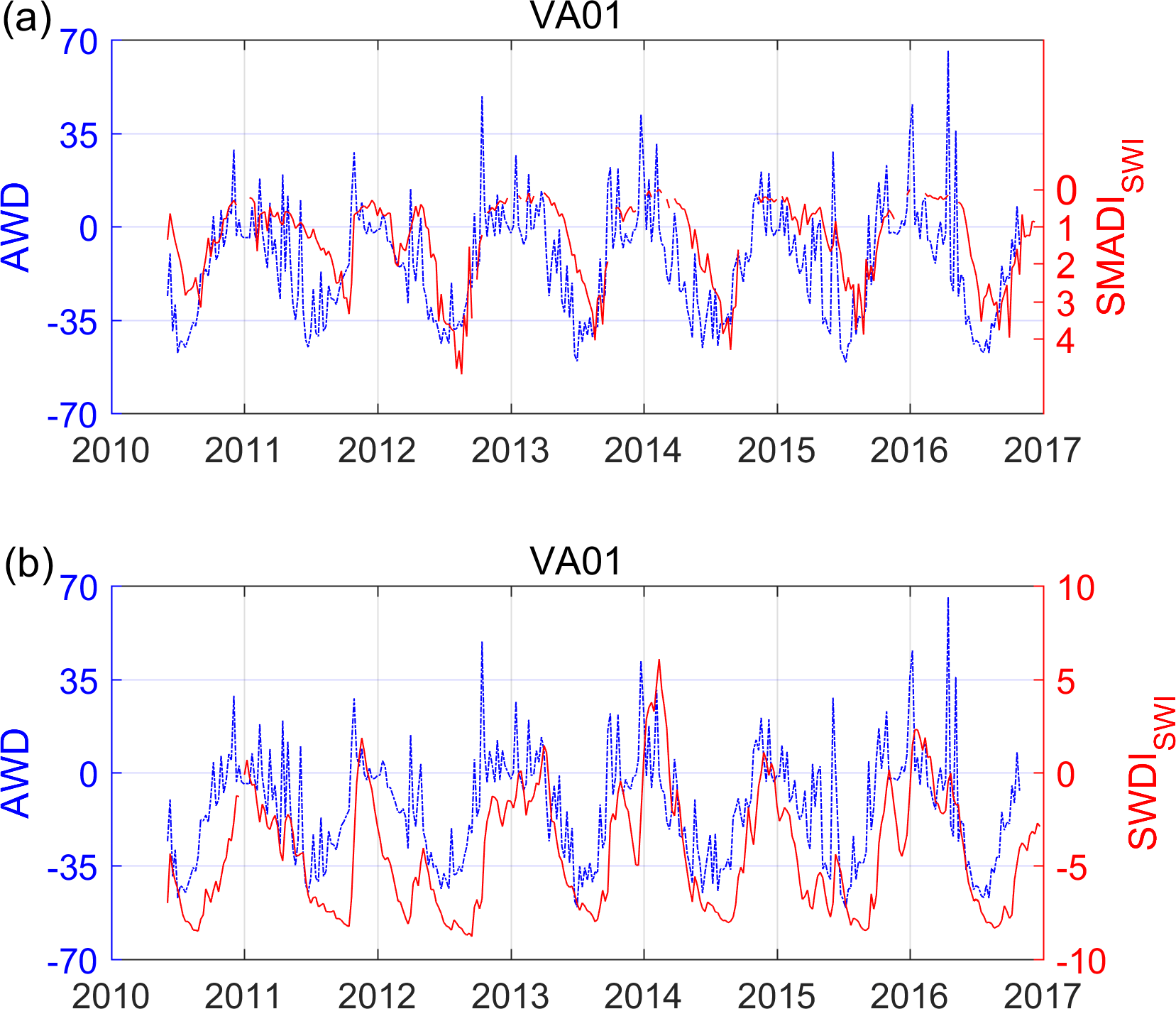
Figure 2 Time series of the weekly AWD and SMADI_SWI (a), and SWDI_SWI (b) at the VA01 station of Inforiego, as an example. Since SMADI =1 and AWD =0 are the threshold for drought (Pablos et al., 2017), both values coincide in the y-axis. In addition, note that the y-axis of SMADI is oriented downward.

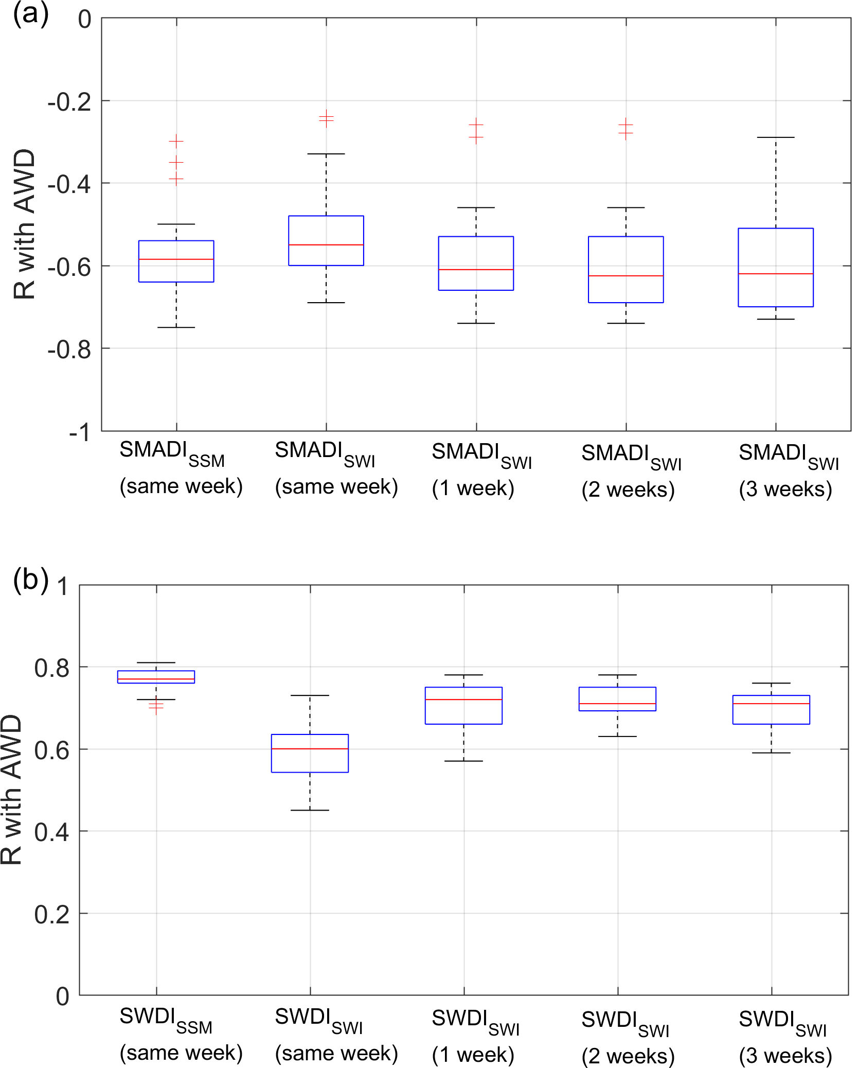
Figure 3 Correlation (R) of the SMADI (a) and the SWDI (b) obtained using the SMOS SSM and SWI, with the AWD of the same week and 1, 2 or 3 antecedent weeks at the 22 Inforiego stations and Villamor. All values were significant (p-value < 0.05).

In general, considering the 25th and 50th percentiles of the boxplots, a delay duration of two weeks obtained the best correlations for both indices. This time lag approximately agrees with the median value of the optimal T over the study area (13 days). Therefore, the SSM-derived indices performed similar degree of agreement with AWD of the same week than that of the SWI-derived indices with AWD of 2 antecedent weeks.

5.2 Comparison with CMI

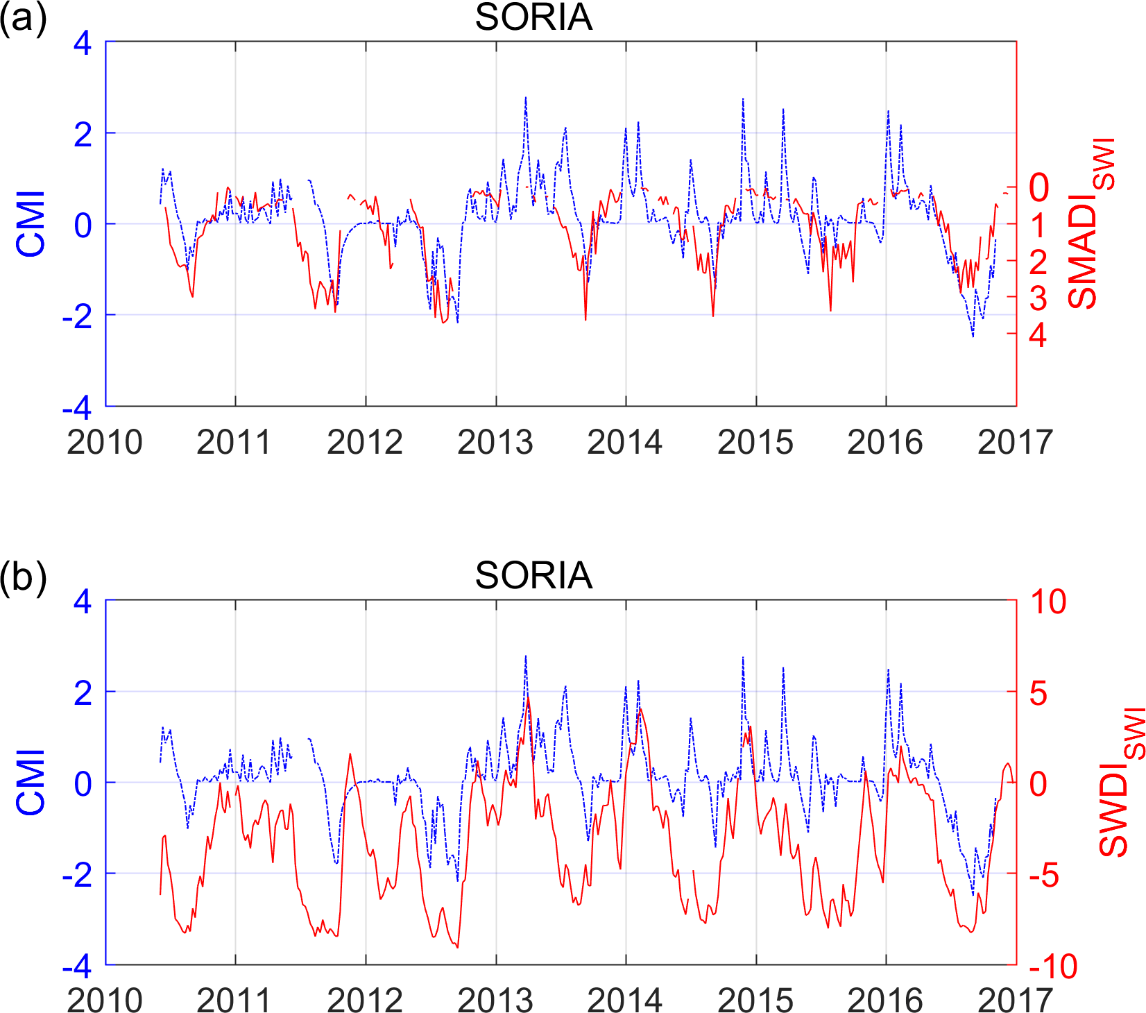
Figure 4 Time series of the weekly CMI and SMADI_SWI (a), and SMDI_SWI (b) at the Soria station of the AEMet, as an example. Since SMADI =1 and CMI =0 are the threshold for drought (Pablos et al., 2017), both values coincide in the y-axis. In addition, note that the y-axis of SMADI is oriented downward.

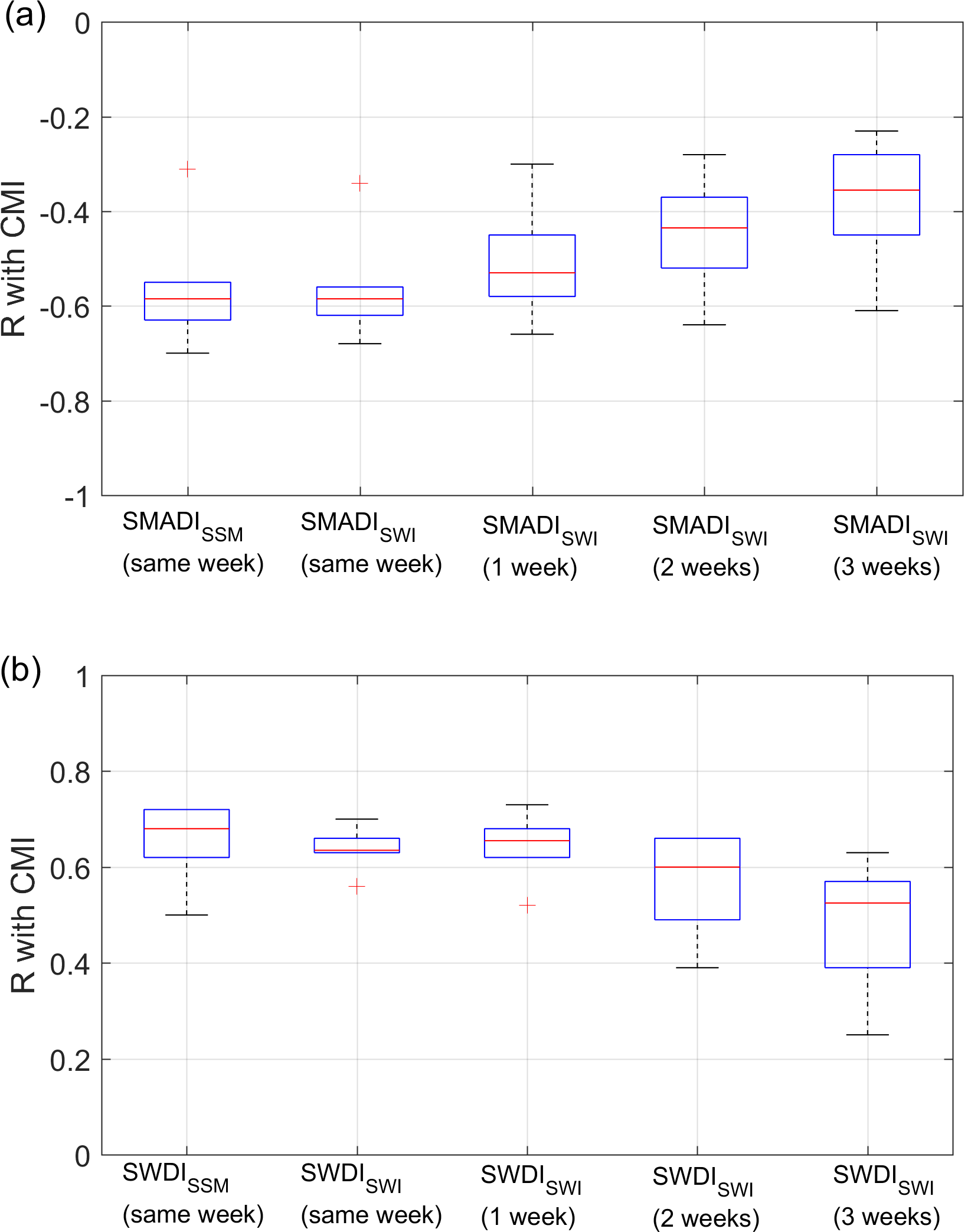
Figure 5 Correlation (R) of the SMADI (a) and SWDI (b) obtained using the SMOS SSM and SWI, with the CMI of the same week and 1, 2 or 3 antecedent weeks at the six AEMet stations. Only significant values (p-value < 0.05) were considered.

The weekly CMI, SMADI_SWI and SWDI_SWI time series at one AEMet station displayed similar seasonal periods (Fig. 4) than AWD in Fig. 2. Note that SMADI was also plotted with its vertical axis increasing downward. However, no delay was observed between the CMI and the SMADI_SWI variations, showing a good correspondence in time (Fig. 4a), as previously found (Pablos et al., 2017; Sánchez et al., 2016, 2018). This could be due to the fact that CMI takes into account the effective soil rooting depth and the soil characteristics, instead of using only climatic data like AWD.

In the case of SWDI_SWI, there were not conclusive results about the existence of a delay in the comparison with CMI (Fig. 4b). As in the case of AWD, previous research showed a time lag between SWDI and CMI when using the in situ RZSM (Martínez-Fernández et al., 2015), but no delay was found when the SMOS SSM was utilized instead (Martínez-Fernández et al., 2016; Pablos et al., 2017). Similar results were obtained at the other AEMet stations of this work (not shown).

The correlation coefficients obtained from the comparison of SMADI_SSM, SMADI_SWI, SWDI_SWI and SWDI_SWI with CMI (Fig. 5) displayed similar results to those discussed in Fig. 4. As in the case of AWD, negative correlation coefficients were obtained between SMADI and CMI, in agreement with their definitions. Both SMOS SSM-derived and SWI-derived SMADI had very similar correlations in the comparison with CMI of the same week (both $R\approx -\mathrm{0.59}$, in median, Fig. 5a). These correlation values decreased in the comparison with CMI of 1, 2, or 3 antecedent weeks ($R\approx -\mathrm{0.54}$, −0.44 and −0.36, respectively, in median). This confirms that SMADI and CMI cycles are synchronized, as observed in Fig. 4a.

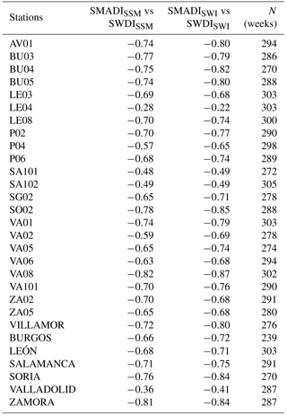
Table 1 Correlation (R) between SMADI_SSM and SWDI_SSM, and between SMADI_SWI and SWDI_SWI. All values were significant (p-value < 0.05). The number of weeks with available data (N) is also included.

When analyzing the correlations of CMI with SWDI (Fig. 5b), the use of the SMOS SWI slightly made decrease the correlation coefficients with respect the use of SSM (R≈0.68 for SWDI_SSM and R≈0.64 for SWDI_SWI, in median). In addition, the correlations between SWDI_SWI and CMI of the antecedent 1, 2 or 3 weeks displayed similar or lower values than when no delay was considered (R≈0.66, 0.60 and 0.30, in median). This result suggests that there is not lag of time between CMI and SWDI_SWI or, if any, the possible duration would be around one week. Nevertheless, further research is needed to assess this issue as well as to evaluate the results with AWD and CMI in other regions with different environmental conditions. During the comparison with CMI, the level of agreement of the SWI-derived indices was similar to that of the SSM-based indices.

5.3 Comparison of SMADI with SWDI

The correlation analysis between SMADI and SWDI clearly showed a high agreement (Table 1), both with SMOS SSM ($R\approx -\mathrm{0.28}$ to −0.82; −0.70 in median) and SWI ($R\approx -\mathrm{0.22}$ to −0.85; −0.74 in median). Additionally, the correlation differences between the SSM and SWI-derived indices were very low (ΔR≈0 to 0.10, in absolute value) to be significant. Thus, the results of both approaches were comparable, as previously observed in the assessment with AWD and CMI. Notwithstanding, in a detailed analysis of the correlation coefficients, 24 out of the total 29 stations obtained stronger correlations in the SWI approach. This suggests a certain trend toward a correlation improvement when the RZSM estimation was used. The high number of weeks with available data (N≈239 to 305 weeks) of a total 342 weeks ensures that the values were robustly computed, as in the previous comparisons with AWD and CMI. However, no conclusions should be inferred from these results because they may hide self-adjustments or other artifacts behind this direct comparison.

6 Conclusions

Since the launch of recent satellite missions dedicated to soil moisture, new applications have been emerged using it as a key agricultural and hydrological variable. Among them, the number of drought approaches is increasing and the results improving. As a great leap forward, several research tries to overcome the drawback of using the soil moisture at surface level derived from remote measurements. With the same aim, two agricultural drought indices, SMADI and SWDI, were applied using remotely sensed soil moisture both at the surface layer (directly retrieved from the sensor observations) and at the root zone (estimated by applying the SWI model to the SSM). The results showed that the use of the RZSM estimation does not influence the characterization of drought through SMADI and SWDI, both in comparison with a meteorological drought index (AWD) and an agricultural one (CMI).

Both SMADI and SWDI showed a similar capability for agricultural drought monitoring, and it was highlighted that a certain time lag should be computed between the at-surface variables (SSM, precipitation) and the RZSM, due to the different response time of the associated processes. This lag is consistent with the SWI model, which takes into account the time lapse of the water transfer from the surface to the deeper soil layers.

The use of RZSM estimations from remote sensing offers a new opportunity for drought monitoring and, in a broadly sense, for many agricultural management applications.

Appendix A: Acronyms

For easy reading of this research, all the acronyms were alphabetically summarized in the following list:

AEMet: Spanish Meteorological Agency

AWD: Available Water Content

AWD: Atmospheric Water Deficit

BEC: Barcelona Expert Centre

CESBIO: Centre d'Etudes Spatiales de la Biosphere

CMI: Crop Moisture Index

DEM: Digital Elevation Model

EASE: Equal Area Scalable Earth

ECMWF: European Centre for Medium-Range Weather Forecasts

ESA: European Space Agency

FC: Field Capacity

ITACyL: Agriculture Technological Institute of Castilla y León

LP DAAC: Land Processes Distributed Active Archive Center

LST: Land Surface Temperature

MODIS: Moderate Resolution Imaging Spectroradiometer

MTCI: Modified Temperature Condition Index

NASA: National Aeronautics and Space Administration

NDVI: Normalized Difference Vegetation Index

NSIDC DAAC: National Snow and Ice Data Center Distributed Active Archive Center

PDSI: Palmer Drought Severity Index

PTF: Pedotransfer Function

REMEDHUS: Soil Moisture Measurements Station Network of the University of Salamanca

RZSM: Root Zone Soil Moisture

SMADI: Soil Moisture Agricultural Drought Index

SMAP: Soil Moisture Active Passive

SMCI: Soil Moisture Condition Index

SMDI: Soil Moisture Deficit Index

SMOS: Soil Moisture and Ocean Salinity

SPI: Standardized Precipitation Index

SSM: Surface Soil Moisture

SWDI: Soil Water Deficit Index

SWI: Soil Water Index

TAW: Total Available Water

VCI: Vegetation Condition Index

WP: Wilting Point