Distributed source pollutant transport module based on BTOPMC: a case study of the Laixi River basin in the Sichuan province of southwest China

Nitrogen and phosphorus concentrations in Chinese river catchments are contributed by agricultural non-point and industrial point sources causing deterioration of river water quality and degradation of ecosystem functioning for a long distance downstream. To evaluate these impacts, a distributed pollutant transport module was developed on the basis of BTOPMC (Block-Wise Use of TOPMODEL with Muskingum-Cunge Method), a grid-based distributed hydrological model, using the water flow routing process of BTOPMC as the carrier of pollutant transport due a direct runoff. The pollutant flux at each grid is simulated based on mass balance of pollutants within the grid and surface water transport of these pollutants occurs between grids in the direction of the water flow on daily time steps. The model was tested in the study area of the Lu county area situated in the Laixi River basin in the Sichuan province of southwest China. The simulated concentrations of nitrogen and phosphorus are compared with the available monthly data at several water quality stations. These results demonstrate a greater pollutant concentration in the beginning of high flow period indicating the main mechanism of pollution transport. From these preliminary results, we suggest that the distributed pollutant transport model can reflect the characteristics of the pollutant transport and reach the expected target.

1 Introduction

The assessment and treatment of watershed water pollution, especially non-point source (NPS) pollution, is currently one of the key environmental protection subjects being addressed by scientists, engineers, and local governments. This is especially true in developing countries like China. According to The Reports on the State of the Environment of China, between 1989–2011, the treatment rate of industrial waste-water and domestic sewage had reached over 90 and 75 %, respectively, until 2010. However, the proportion of monitored sections for water quality beyond Class III in the 7 stream networks (including 469 state-level sections) and main lakes (including 26 state-level sections) of China was still as high as 40.1 and 80.8 %. These data indicates that PS pollution has been controlled effectively in China during the last more than ten years but NPS pollution are still very serious and has become the dominant pollution source leading to over-standard water quality. This is caused by the characteristics of NPS, such as the dispersion, uneven spatial and temporal distribution, randomness, long incubation period, and the difficulty for monitoring and controlling relative to PS pollution (Wu et al., 2006; Nigussie et al., 2003; Hao et al., 2006). The complicated mechanism of NPS decides that it is very difficult to simulate and evaluate NPS quantitatively and accurately.

The assessment models for NPS pollution can be categorized into two types – the empirical model and the mechanism model (Nash et al., 1970; Beven et al., 1979; Jiang et al., 2011). The empirical models are built on the basis of empirical relationships between watershed physiographic characteristics and pollutant exports, such as the Export Coefficient Method (Johnes and Heathwaite, 1996; Johnes and O'Sullivan, 1989) and Source Strength Coefficient Method (SSCM) (Chinese Academy for Environmental Planning, 2003). In general the empirical models have a lower simulating accuracy, but they are usually applicable enough for many practical applications like the watershed water pollution treatment, water environmental impact assessments, water environmental planning and etc. In comparison, the mechanism models generally have stronger simulating ability than the empirical models. There are many good NPS models developed on some mechanism of pollutant transport and transformation, such as the Hydrological Simulation Program–Fortran (HSPF), Soil and Water Analysis Tools (SWAT), Better Assessment Science Integrating Point and Non Point Sources (BASIN) (Nasr et al., 2007; Anderton et al., 2002; Orth et al., 2015) and etc., which can simulate the physical, chemical, and biochemical processes in some extent and to estimate the effects of agricultural management measures and practices (USEPA, 2000). Mechanism model has some advantages compared with empirical model like the higher accuracy, clear principles, parameter portability between different catchments and great development potential; however, its complex mechanism requires the more accurate and larger amount of input data which makes it very difficult to apply in the small basins or the basins without enough monitoring data (Andréassian et al., 2009; Cho et al., 2008; Jiang et al., 2011), especially in the developing countries which has poor monitoring data of hydrological and meteorological observation data (Kobierska et al., 2013; Singh et al., 2014; Ying et al., 2010).

Certainly, the mechanism model has become the main area of NPS study and will has great development and application in the future accompanying with our deeper and more understanding to the NPS mechanism, the increasing of the observation data and the development of observation techniques and equipments. However, due to the scarcity of observation data and sites, the empirical NPS model is still widely applied in the ungauged basins (PUB) and regions (Bookera and Woods, 2014; Viviroli et al., 2009; Ying et al., 2010). And with the economic progress, more and more developing countries and regions have the serious water pollution issue, which have urgent and pressing need to evaluate and control the NPS although they have poor observation data of hydrological, meteorological and water quality observation data and equipments.

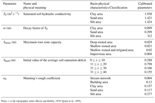
Based on the advantages of mechanism model and the actual situation of ungauged basins and regions: the scarcity of observation data and sites and the wide application of empirical models, this study developed a distributed source pollutant transport module (DSPTM) based on a grid-based distributed hydrological model, BTOPMC and the empirical NPS assessment model, the Export Coefficient Method, to simulate the NPS pollutant transport process with the direct runoff and evaluate the contribution of NPS and the impact of the direct runoff on the N and P concentration at the monitored sections and applied it in the study area of the Lu county area situated in the Laixi River basin in the Sichuan province of southwest China.

2 Methodology

2.1 The NPS transport mechanism in DSPTM

BTOPMC (referred to as the Yamanashi Hydrological Model (YHyM) in Japan) is a grid-based distributed hydrological model, developed in Yamanashi University in the 1990s (Ao et al., 2003; Takeuchi et al., 2008) and applied widely around the world, with good impacts and research value (Bao et al., 2010; Takeuchi et al., 2013; Yoshimura et al., 2010). It has been applied particularly in areas with warm, humid climates and with high elevations and sloping landscapes, such as Japan and Southeast Asian countries (Zhou et al., 2006; Yoshimura et al., 2007, 2010; Reichert et al., 2001; Ao et al., 2006; Takeuchi et al., 1999). BTOPMC has five calibrating and validating model parameters–saturated soil hydraulic conductivity (T₀), decay factor of T₀ (m), maximum root zone capacity (S_rmax), initial value of the average soil saturation deficit (S_bar0), and Manning's rough coefficient (n₀) (Ao et al., 2003; Takeuchi et al., 1999).

The DSPTM is a distributed source pollutant module developed on the BTOPMC and implanted into the BTOPMC as an extension of its function (Fig. 1). The basic principles of the model include the mass balance of pollutants within the grid and the pollutant transmission between grids along the runoff direction. According to the research findings, the transport and transformation of pollutants are carried by runoff. In this study, the concentration process of BTOPMC was treated as the carrier of the pollutant transport. The BTOPMC model is a grid-based distributed hydrological model. The basin is segmented into a rectangular grid net and the runoff yield and concentration processes are calculated in each rectangular grid for each time interval. The concentration mechanism of BTOPMC is based on the Muskingum-Cunge Method which is used for the concentration calculation of each grid. The concentration calculation was applied grid by grid, successively along the runoff direction, until the control section grids were reached. Simultaneously, the pollutant was transferred along the runoff route of the concentration for each time interval, and the mass balance for pollutants within each grid was calculated (Eq. 1). In this way, the pollutant flux through each grid including the control section grid was calculated for each time interval.

In BTOPMC, the basin grids are divided into two types – the slop grid and the river grid by setting the area threshold of the upstream catchment of each grid. The NPS pollutant transport module for the slop grid and river grid is built on the basis of two basic principles – the mass balance for each pollutant within each grid and the pollutant transmission between grids along the runoff route of the concentration. The module includes 5 variables of pollutant input and output: (1) pollutant mass within the grid at the beginning of the period WP_ini(t); (2) pollutant mass within the grid at the end of the period WP_end(t); (3) pollutant input mass from the upstream grids for each time interval ∑WP_in(t). (Because it is similar to the concentration process, a grid might receive pollutant input from several upstream grids.) (4) Total pollutant mass from the direct input (NPS pollutants for slop grids and PS pollutant for river grids which were set as the PS input grids) ∑WP_{direct_in}(t); (5) pollutant output mass to the downstream grid TN_out(t). Pollutant mass conservation within a grid is shown in the following formula:

$$\begin{array}{}\text{(1)}& {\displaystyle }\begin{array}{l}\mathrm{\Delta }\mathrm{WP}={\mathrm{WP}}_{\mathrm{end}}-{\mathrm{WP}}_{\mathrm{ini}}\\ =C_{\mathrm{WP}\mathrm{\_}\mathrm{end}}{V}_{\mathrm{end}}-C_{\mathrm{WP}\mathrm{\_}\mathrm{ini}}{V}_{\mathrm{ini}}\\ =\sum {\mathrm{WP}}_{\mathrm{in}}+\sum {\mathrm{WP}}_{\mathrm{direct}\mathrm{\_}\mathrm{in}}-{\mathrm{WP}}_{\mathrm{out}}\end{array}\end{array}$$

where ΔWP: Pollutant mass increase within the grid for each time interval, t; C_{WP_ini}: Pollutant concentration at the beginning of the time interval, mg L⁻¹; C_{WP_end}: Pollutant concentration at the end of the time interval, mg L⁻¹; V_ini: Water storage within grids at the beginning of the time interval, m³; V_end: Water storage within grids at the end of the time interval, m³.

2.2 Assumptions of the pollutant load in grids

Due to the scarcity of observation data, the annual total nitrogen (TN) and total phosphorous (TP) load of different land-use area of study area has been estimated by the Export Coefficient Method in the earlier study (Zhang et al., 2013). Therefore, based on the characteristic of local residents treating the domestic wastes, the starting-stage situation of model study and the NPS accumulation law, this study has three assumptions for the pollutant load in grids.

In the rural and town area of southern China, the domestic sewages like the livestock and poultry waste are usually treated with the biogas tank or septic tanks then returned to the farmland as a fertilizer anytime and it is difficult to understand the accurate time law of wastes entering the fields. So this study assumed that the load entering into the study area is uniform daily in the study period (Assumption (1): load temporal distribution), the load into the same land -use grids is uniform in the spatial distribution (Assumption (2): load spatial distribution) and the load will be accumulated when no runoff in this grid and brought to the downstream grid when there is runoff in the grid (Assumption (3): load accumulation).

Figure 1 Framework of NPS pollutant transport module.

3 Data of study area

3.1 Basic information of study area

The study area, the Lu County area of Laixi River basin, with a drainage area of 728 km², is located in Sichuan province in southwest China at 105^∘14^′57${}^{\prime \prime }$–105^∘41^′51${}^{\prime \prime }$ E, 28^∘59^′56${}^{\prime \prime }$–29^∘20^′3${}^{\prime \prime }$ N (Fig. 2). It includes three main rivers. The Lu County reach of the Laixi River and its two branches – Jiuqu River and Maxi River, have a total length of 130 km. The Laixi River has a basin area of 3257 km², is one of the two main tributaries of the Tuo River of the upper Yangtze stream networks, and originates from Dazu district of Chongqing city and flows into the Tuo River in Hushi town of Luzhou city, Sichuan province.

The study basin has a humid subtropical climate with an average annual precipitation of 991.7 mm and reference evaporation of 980 mm. The mean annual temperature is 17.7^∘, and there is a large mean temperature difference of 19.2^∘ between winter and summer. There is heavy forest coverage, and, until 2010, it covered 39.5 % of the area. The dominant terrain type is hills, which cover nearly 87.5 % of the study area, and incline towards the southwest with elevations ranging from 218 to 757.5 m and an average slope of 8 %. The dominant land use types are the paddy field and dry land, with a total ratio of 69 % of study area, which means that most of the area is used as agricultural land and agricultural NPS pollution will be a serious a result of the heavy utilization of the fertilizer and pesticides.

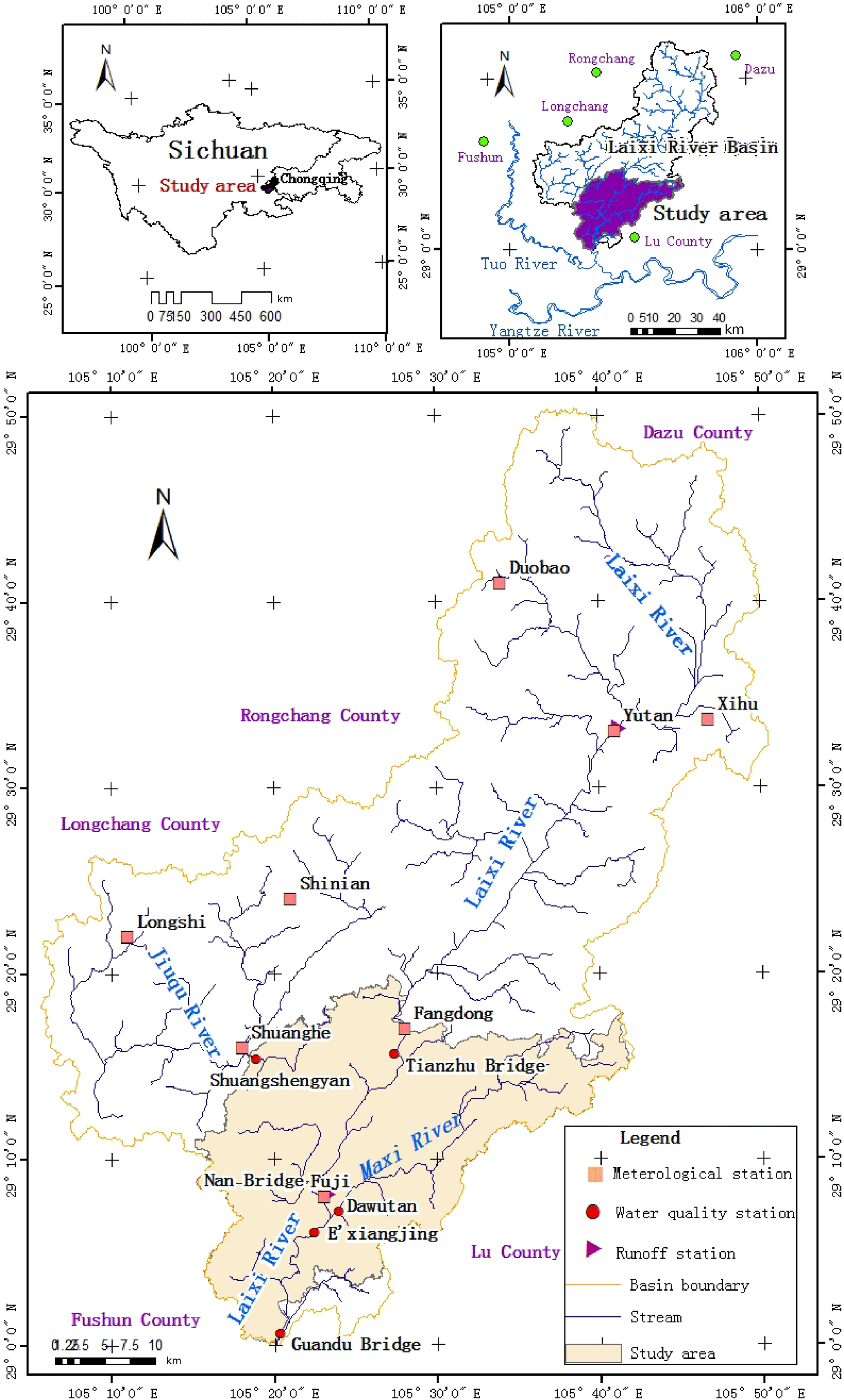
Figure 2 Study area and the spatial distribution of hydrological, meteorological, and water quality stations.

The Study area includes 10 towns and 157 villages, with an urban population of 73 775 and an agricultural population of 472 504 (about 85 % of the total population). There is only one sewage treatment plant until 2011, located in Fuji Town, which has a daily treatment capacity of 6000 t (equal to the daily domestic sewage amount for about 17 911 persons). Therefore, except a part of the domestic sewage from Fuji Town, which is treated by the Fuji sewage treatment plant and discharged into the stream networks as the Discharge Standard of the Pollutants for Municipal Wastewater Treatment Plant (GB18918-2002), the other domestic sewage from Fuji and the other towns (including both the agricultural population and nonagricultural population) is only treated with septic tanks or biogas tanks. These results in livestock and poultry waste being discharged into the simple septic tanks, which are usually dug out in the ground, and then returned to the farmland as a fertilizer when the septic tank is full. In large-scale livestock and poultry farms waste will be treated with a biogas tank anaerobic system, and then the biogas slurry and residue from the waste will similarly be returned to farmland. In the study area, there are many industrial plants, including wine plants, paper mills, chemical plants, and glass factories, which are the major source of PS pollution.

3.2 The related data for DSPTM application

1. DEM, land use/land cover and soil data
   The Digital Elevation Model (DEM) of the study area was obtained from the Soil and Sources Bureau of Sichuan Lu County, with the accuracy of 30 m. Soil types and their distribution data (1000 m) were download from the Food and Agriculture Organization of the United Nations (FAO). Land use/land cover data (30 m) were collected from the Second Land and Resources Investigation of China.

2. Hydrological and meteorological data
   Hydrological and meteorological data were collected from local hydrological and meteorological governmental sectors. The eight Rainfall stations that were used were Xihu, Duobao, Yutan, Fangdong, Longshi, Shinian, Shuanghe, and Fuji (Fig. 2), with daily rainfall from 1979–1987 and 2011. The two evaporation stations that were used were Dengying and Guanyin(2^∗), with monthly evaporation data from 1979–1987 and 2011. The two runoff stations used were the Fuji station and Yutan station, both with daily rainfall data from 1979–1987 and 2011 (Fig. 2).

3. Water quality, PS and NPS pollution data
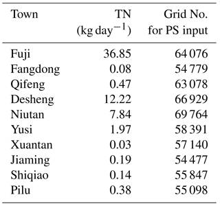
   Population and animal data were derived from local government sectors and a field survey of the local committees of the village, farmers, and scientific and technical personnel. Water quality data were collected from the environmental protection administration of Lu County. The six water quaity monitoring sections that were used were the Tianzhusi, E'xiangjing and Guandu Bridge station in the Laixi River (3 stations); Shuangshengyan and Nan Bridge in Jiuqu River (2 stations) and Dawutan in Maxi River (1 station) (Fig. 2). The study area has the monthly water quality data of 2011, with 22 monitoring factors including ammonia nitrogen (NH${}_{\mathrm{4}}^{+}$-N), TN, and TP, among others. Two pollutant indicators were TN and TP and the six pollution sources were natural woodland source, rural NPS (agricultural NPS, rural and town domestic sewage, livestock and poultry source), construction land source and industry waste-water source (PS).

   Based on the annual pollutant load of each land-use type estimated in the earlier study and the assumption (1) and (2), the daily load of each grid from three land use of natural land, farmland and impervious surface is calculated (Table 1 and Fig. 3). The industry waste-water source (PS) is allocated into the PS input grids. As there was no TP data for the industry waste-water source, the PS input only included TN input (Table 2 and Fig. 3).

Figure 3 Reclassified land use and PS pollution input grid distribution.

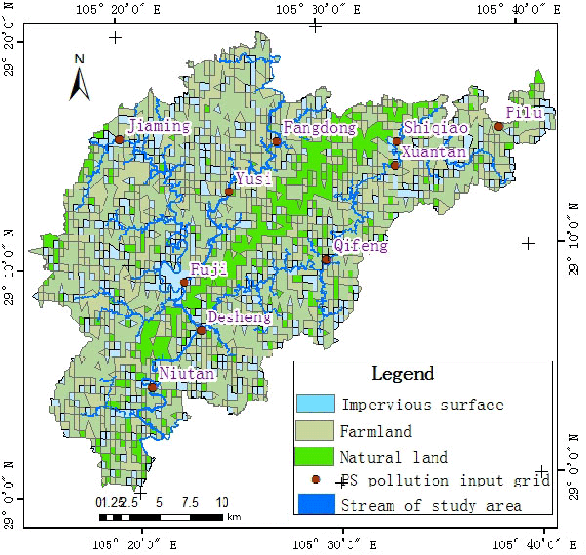
Table 1 Pollutant daily input amount for each land-use grid Units: kg/grid/day.

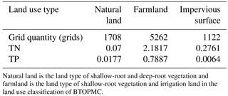
Natural land is the land type of shallow-root and deep-root vegetation and farmland is the land type of shallow-root vegetation and irrigation land in the land use classification of BTOPMC.

Table 2 Daily river pollution load and PS input grid No. for industry waste-water source (PS) of each town.

4 The application of DSPTM in study area

The application for DSPTM includes two steps – the calibration and validation stage for BTOPMC and the application stage for DSPTM. As the carrier of the pollutant transport, the BTOPMC was calibrated and validated first, and then the DSPTM was applied in the study area.

4.1 The calibration and validation for hydrological model, BTOPMC

The calibration and validation information for the BTOPMC model parameters can be seen in Tables 3 and 4. The calibration and validation effect meets the requirements, with the Nash-Sutcliffe efficient as 57.46 % for calibration and 65.36 % for validation.

Table 3 Calibration and validation information for BTOPMC model parameters.

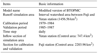
Table 4 Calibrated model parameters for BTOPMC.

Notes: λ is the topographic index (Beven and Kirkby, 1979; Quinn et al., 1995).

4.2 The application of DSPTM in study area

The DSPTM was applied in the Lu county area of Laixi river basin with the data of 2011. According to the spatial distribution of the water quality monitoring sections, the three sections of Tianzhusi, Shuangshengyan, and Dawutan were set as the inflow water quality monitoring sections of the study area (Fig. 2). Therefore, in the NPS pollutant transport simulation, the measured pollutant concentration of the three inflow sections was used to replace the pollutant concentration of the corresponding river grids, to simulate the pollutant concentration of Nan Bridge, E'xiangjing, and Guandu Bridge for each simulation interval. The time step for simulating pollutant concentration in this study is daily, but the monitoring time step of the measured data is monthly. The change of the water quality is gradual when there are no sudden water quality events. Therefore, the monthly measured values of water quality monitoring sections were converted into daily pollutant concentrations by the temporal linear interpolation method (Table 5).

In addtion, the model was intialized like this (Starting time: 1 January 2011): (1) Initial concentration of river channel grids. Pollutant initial concentration of river channel grids can be calculated through the spatial linear interpolation of the measured concentration values of water quality monitoring sections on the starting time. (2) Initial concentration of slope grids. The study assumed that initial pollutant concentration of slope grids was zero and the pollutant concentration of slope grids was zero when there was no runoff (The grid outflow is smaller than 0.01 m³/s).

Table 5 Basic information for DSPTM application.

4.3 Results

In this study, the 2011 daily observed water quality data of Nan Bridge, E'xiangjing, and Guandu Bridge sections were used to test the performance of DSPTM with two pollution indicators of TN and TP. The TN and TP graphs of the three control sections are shown in Fig. 4a–f. Meanwhile, the model prints the spatial distribution of TN on 1 July (wet season) and 1 February (dry season), see Fig. 6. Overall, the simulated results are as expected.

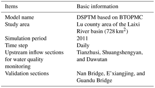
1. The simulated and measured values for annual pollutant flux of the control sections (Nan Bridge, E'xiangjing, and Guandu Bridge) are close to each other. The results of comparisons between the simulated and measured value showed that for 2011 TN and TP pollutant flux of the control sections, the relative errors are within 10 % of one another and close to 10 %, respectively. The simulation relative error for the TN pollutant flux of the Guandu Bridge is slightly larger, at nearly 11.34 %. The relative error of the other control sections can be seen in Table 6. This indicates that the simulation effect for the annual pollutant load amount of study area is generally not bad.

2. The statistics indicators of Nash-suttcliffe coefficient and Mean relative errors shows that the simulation effect of the concentration variation process is bad (Table 6). As shown in Fig. 4a–f, for the 2011 TN and TP daily concentrations of the three control sections, the simulation and measured process graphs display a uniform variance trend and the simulated values fall around the measured values, within a certain range. This indicates that the simulation results can reflect the temporal change trend of pollutant concentration for control sections but the simulation values have poor performance, especially at peak concentration. This is because assumptions (1) and (2) cannot reflect the actual concentration distribution. In further studies the temporal and spatial distribution simulation for NPS pollutants will be the research emphasis.

3. The simulation results show that the pollutants concentration in the beginning of the flood period is slightly greater, which is in accordance with the characteristics of the NPS pollution generating process. This indicates that assumption (3) is reasonable. By analyzing the concentration peak and the process grphs for TN and TP of the control sections, the following features can be found: (a) Pollutant concentration peaks typically occur at the end of April or the beginning of May, which marks the beginning of the flood period; (b) With the flood period continuing, the pollutant concentration decreases gradually and tends to be stable; (c) At the beginning of November, the dry period, the pollutant concentration increases slightly. The above features reflect the characteristics of the occurrence of NPS pollution. Before the flood period, pollutants accumulate on the ground surface due to the weak driving force from rainfall and runoff. With the beginning of the flood period, the accumulated pollutants are carried off and migrated by the runoff and afflux into the river. That is why river pollutant concentration increases at the beginning of the flood period. NPS pollution refers to the phenomenon that the dispersive pollutants on ground surface are carried and migrated into river. With the continuous scouring for pollutants on the ground surface with runoff, the accumulated pollutant amount decreases gradually, which cause the reduction in the generating intensity of NPS. Meanwhile, the river pollutant concentration also decreases gradually and tends to be stable. During the dry period, although there is no NPS pollution and PS pollutants are the main pollution sources, the river pollutant concentration increases slightly because the river flow is relatively small. The above analysis demonstrates that assumption (3) is reasonable to some extent.

4. The spatial distribution of TN on the wet and dry season shows that a large amount of NPS pollutant is accumulated on the slope grids of the study area on the dry season and the pollutant is brought away with the direct runoff on the wet season (Fig. 5). That meets the transport feature of NPS.

Table 6 Pollutant flux for TN and TP of controlling sections and their relative errors.

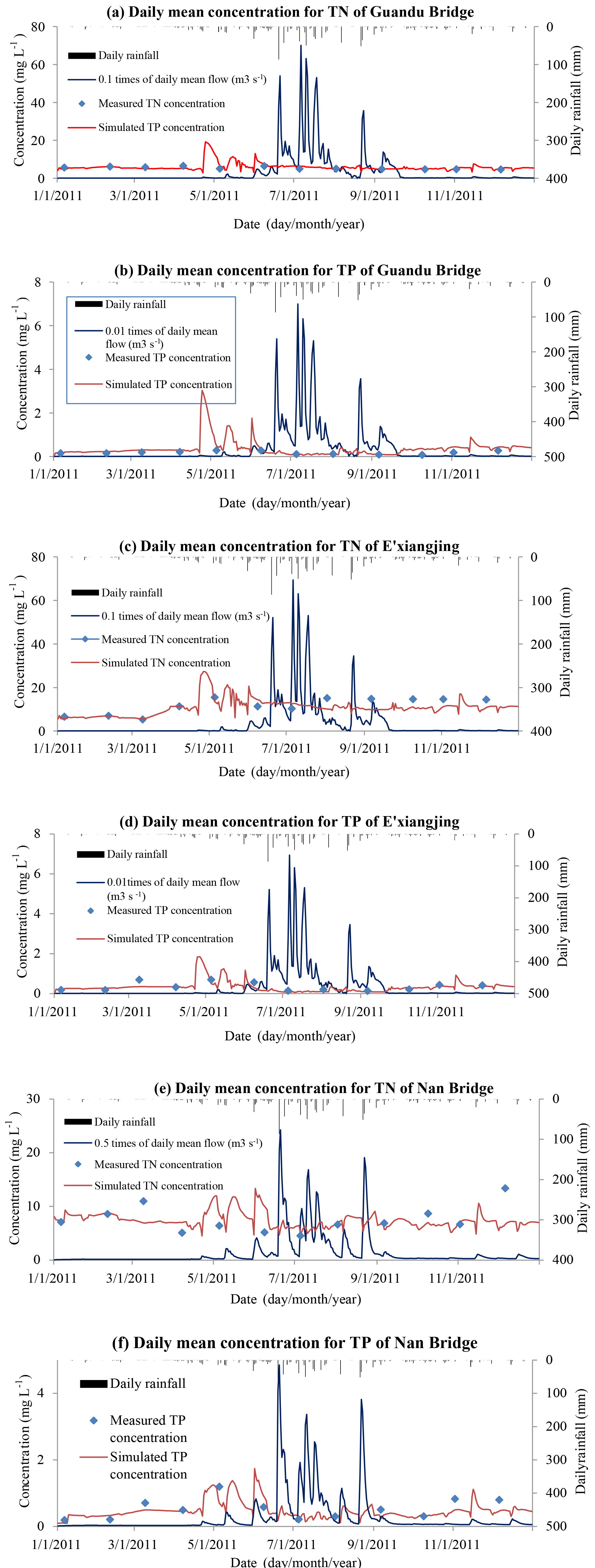
Figure 4 (a)–(f) Daily mean concentration for TN and TP of Guandu Bridge, TN and TP of E'xiangjing and TN and TP of Nan Bridge.

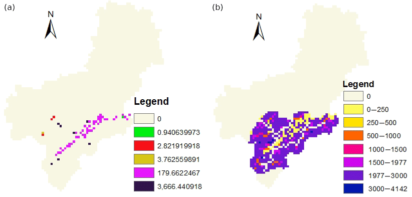
Figure 5 The spatial distribution of TN on 1 July (a, wet season) and 1 February (b, dry season), kg.

5 Summary and conclusion

This study aimed to develop a distributed NPS simulation model based on BTOPMC. This study developed a DSPTM based on the concentration process of BTOPMC. Runoff is the carrier of pollutant transport and transformation in catchment. The basic principles of DSPTM include the mass balance of pollutants within a grid and the pollutant transmission between grids along the runoff direction in catchment. The grids in catchment were divided into slope grid and river channel grid, therefore, the transport process was divided into two stages of slope pollutant transport and river channel pollutant transport. For slope transport process, NPS, such as natural woodland source, rural NPS and construction land source, are the dominant pollution sources. For river channel grids, the dominant pollution source is PS, i.e. industrial waste-water source.

In this model application, the pollution source data derived from earlier results from the study area, which were calculated using the Export Coefficient Method. Any errors in the earlier study results would influence the accuracy of the DSPTM simulated results. Because of the shortage of hydrological and environmental data, the Lu County area of the Laixi river basin was selected as the study area; this area is not an integrated watershed. Three upstream sections of the study area, Tianzhusi, Shuangshengyan, and Dawutan, were set as the pollutant input sections, which made the modeling process complicated. The measured errors of the water quality data of the three sections could have increased errors in the simulated results. The runoff parameters of BTOPMC were calibrated and validated in the integrated Laixi basin, so they would not influence the results of water quality simulation.

To fit the DSPTM test, three assumptions – the even distribution of NPS pollutants in temporal and spatial scale and the pollutant accumulation within the grids where there is no runoff, were proposed. We found that the first two assumptions could not reflect the actual pollutant distribution in the basin, which lead to a bad fitting effect of the simulated and measured pollutant concentration. However, according to the simulated results, including the time accordance of pollutant concentration peak with the flood peak assumption 3 was confirmed to be reasonable.

Overall, the simulated results show that DSPTM can, to some extent, reflect the characteristics of NPS pollutant transport and reach the expected target. In further studies, the pollutant distribution mode in space and time and the pollutant generating model will be developed to improve the simulated results.