Temporal and spatial distributions of flood water storage volume of the main river and tributaries in the Ishikari River basin

In recent years, Japan experienced frequent and intense heavy rainfalls, resulting in serious flood disasters in many areas. It is also necessary to control floods in tributaries and basins of these tributaries in addition to flood control of the main river. This will be accomplished by understanding flood formation process in the basins of tributaries as well as the main river. Integrated flood flow analysis for the main river and tributaries was conducted by the use of observed temporal changes in the water surface profiles of the 2016 flood in the Ishikari River, Hokkaido, Japan. Temporal and spatial water storage volume distributions in the Chitose River and Ishikari River basins give a new graphical representative method to visualize that when, where, how much volume of rainfall are stored in each basin, and make it possible to verify effects of flood control measures.

1 Introduction

In recent years, Japan experienced frequent and intense heavy rainfalls, resulting in serious flood disasters. To have an integrated flood control plan of the entire basin including the main river and tributaries is important for reducing effectively flood disasters. For this purpose, it is essential to estimate the flood flow dynamics in the main river and tributaries. There are two analysis methods for such studies: hydrological rainfall-runoff analysis and hydraulic flood flow analysis.

The former is a method for mainly representing the runoff mechanism of rainfall and estimating the discharge. The storage function method (Kimura, 1961; Hoshi and Yamaoka, 1982), tank models (Sugawara, 1972; Gotoh et al., 2019), and distributed models (Tachikawa et al., 2004) considering rainfall distribution and topographical and geological characteristics are used to estimate runoff discharge.

On the latter method, Fukuoka et al. (2004) proposed 2D flood flow analysis method to obtain flow velocity distributions and flood flow discharge hydrographs at any point in rives. Fukuoka (2017) also estimated the temporal and spatial distributions of water storage volume in the upstream basin, dams, rivers, and inundation area in the September 2015 flooding of the Kinu River basin and visualized water storage volumes in the basin. Mikami et al. (2021) evaluated effects of the discharge hydrographs of the primary and secondary tributaries on the flood discharge of the main river in the upper Tone River basin by 2D flood flow analysis.

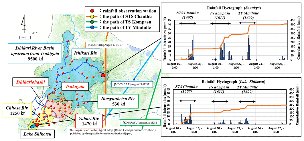
Figure 1 Basin map of the Ishikari River and the Chitose River and the rainfall hyetographs at the main stations in the upper Ishikari River basin and the Chitose River basin.

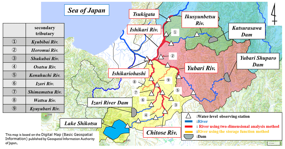
Figure 2 Basin map of the lower Ishikari River.

In this study, analysis of flood flow of the 2016 typhoon was conducted to obtain the water surface profiles over time for the main river and tributaries in the lower Ishikari River basin shown in Figs. 1 and 2. The discharges from most of secondary tributaries are estimated by using the storage function method by Hoshi and Yamaoka (1982). We first examined characteristics of the three flood flows of 2016 typhoon and the effects of the discharge hydrographs in the Chitose River basin on the Ishikari River. Then, the temporal and spatial water storage volume distributions in each tributary and entire basin are discussed.

2 Characteristics of river basin and rainfall

The Ishikari River has the second largest basin in Japan and consist of a large number of tributaries. The Ikusyunbetsu River, Yubari River, and Chitose River are primary tributaries and confluent in the lower Ishikari River reach between Ishikariohashi (25 km from the river mouth, hereinafter shown as KP25) and Iwamizawaohashi (KP45). There are 83 rainfall observation stations in the lower Ishikari River basin as shown in Fig. 1. The hyetographs at the main stations in the upper Ishikari River basin and the Chitose River basin are also shown in Fig. 1. STS Chanthu, TS Kompasu, and TY Mindulle which are the names of typhoons hit Hokkaido during 17–23 August 2016, and brought successively extensive disasters in the Ishikari River basin. The three typhoons took different paths, resulting in different rainfall distributions. STS Chanthu brought the rain exceeding 20 mm h⁻¹ in the Chitose River basin and TS Kompasu and TY Mindulle did the peak rain about 25 mm h⁻¹ in the upper basin of the Ishikari River basin.

Figure 3 Flood surface profile of the Ishikari River in STS Chanthu.

Figure 4 Flood surface profile of the Chitose River in STS Chanthu.

Figure 5 Flood surface profile of the Ishikari River in TS Kompasu.

3 Analysis method

3.1 Flood flow analysis in the main river and primary tributaries

Parts of red line shown in Fig. 2 are river reaches analysed in the 2D flood flow analysis so as to match the observed water surface profiles. The upstream boundary condition for the analysis was given by observed water level. Velocity profiles were then calculated at each cross-section. The discharge hydrograph was obtained from calculated velocity distributions and channel area during flood.

3.2 Calculation method of runoff discharge in secondary tributaries

Flood flows of the secondary tributaries coloured by red in Fig. 2 were analysed in the same way as the flood calculation of the main and primary rivers. However, for the secondary tributaries coloured by orange in Fig. 2, water level data was not available because there were not water-level observation stations. Therefore, runoff volumes from such tributaries were estimated by the storage function method (Hoshi and Yamaoka, 1982) and added as lateral inflow to the 2D flood flow analysis. The residual areas were not included in the lateral inflow because their areas are very small.

4 Analysis results

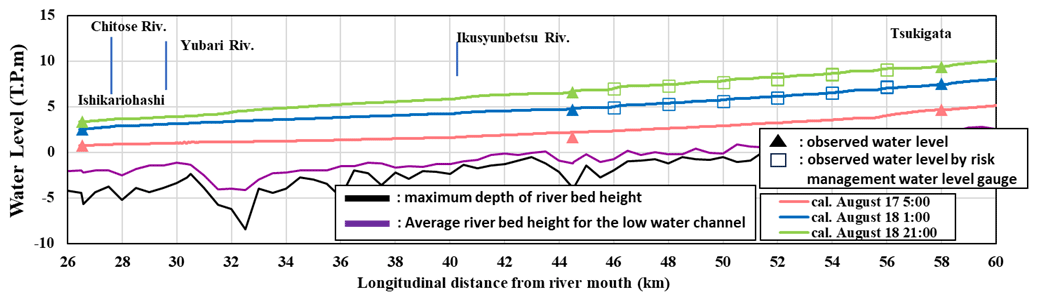
Figure 3 shows the temporal variations of the water surface profiles of the Ishikari River floods due to STS Chanthu. Figure 4 also shows the temporal variations of the water surface profiles of the Chitose River. The peak discharge of Ishikari River occurred at 21:00 JST (Japan Standard Time), 18 August. On the other hand, the Chitose River reached its peak at 01:00 JST, 18 August. Backwaters from the Ishikari River to the Chitose River are comparatively small at the peak time.

Figure 6 Flood surface profile of the Chitose River in TS Kompasu.

Figure 7 Discharge hydrograph of the Ishikari River.

Figure 8 Discharge hydrograph of the Chitose River.

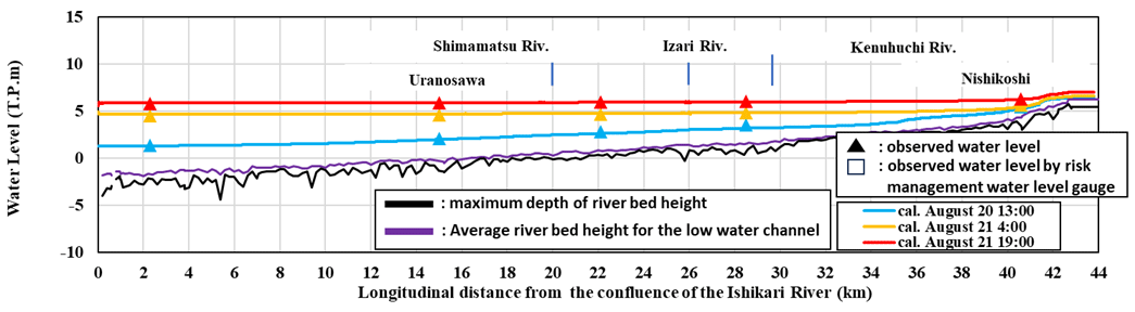
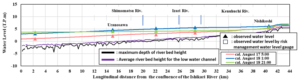
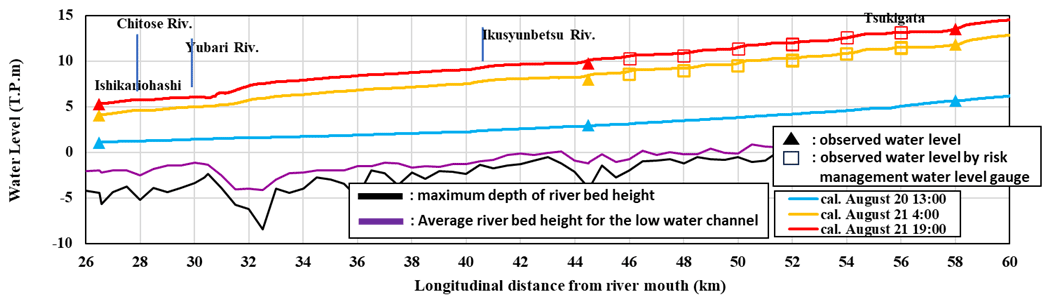
TS Kompasu brought more rainfall in the upper reach of the Ishikari River than STS Chanthu. Figure 5 shows that the peak water level of the Ishikari River of TS Kompasu is higher than that of STS Chanthu. Figure 6 shows that the water level of the Chitose River is also rising due to the rise of water level of the Ishikari River (backwater). In particular, at 19:00 JST, 21 August, the backwater reaches up to 40 km from the confluence of the Ishikari River.

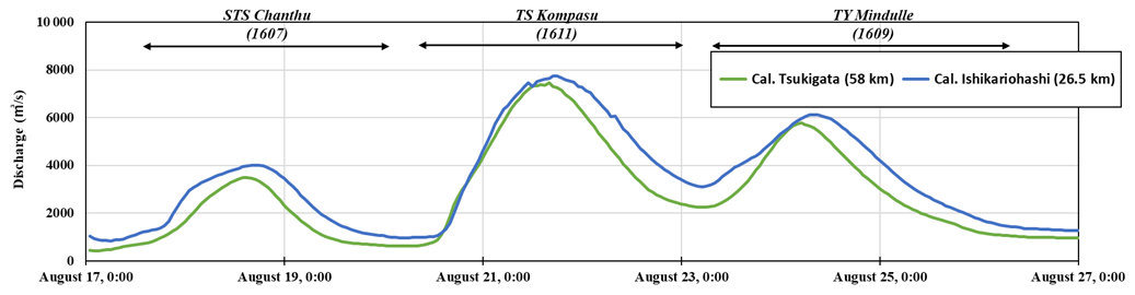
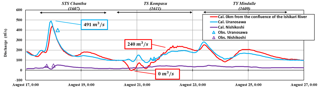
The discharge hydrographs of the Ishikari River are shown in Fig. 7. The calculated discharge hydrograph and the observed discharge at two stations of the Chitose River are compared in Fig. 8. STS Chanthu brought heavy rainfalls in the Chitose River basin, and the peak of flood flows of the Chitose River occurred about 1 h before of the Ishikari River. In particular, the peak at 01:00 JST, 18 August was 491 m³ s⁻¹ at Uranosawa.

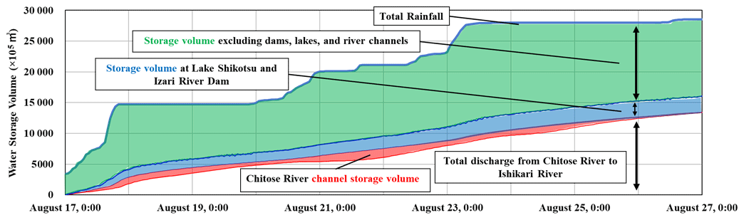
Figure 9 Graphical representation of temporal and spatial water storage volume distributions in the Chitose River basin.

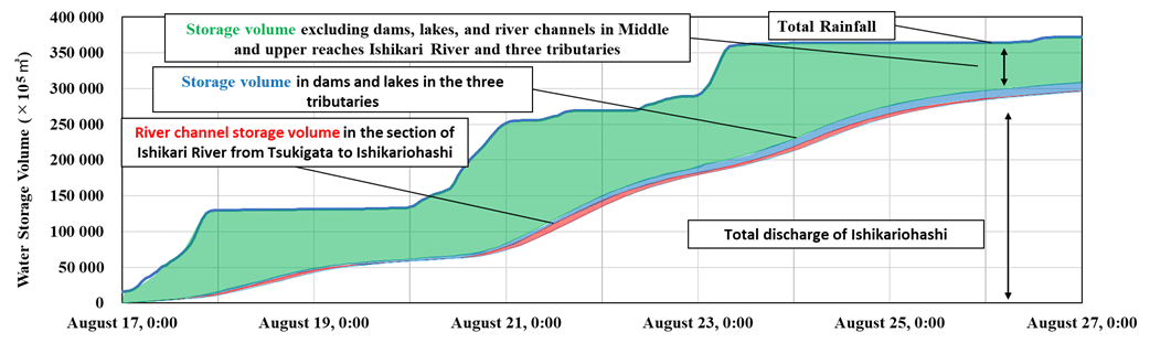
Figure 10 Graphical representation of temporal and spatial water storage volume distributions in the Ishikari River basin.

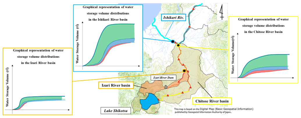
Figure 11 Graphical representations of temporal and spatial water storage volume distributions in each basin on the basin map.

In the second, the Chitose River are strongly influenced by the backwater of the Ishikari River. At 19:00 JST, 21 August, the peak discharge time of the Ishikari River, the discharge at 0 km from the confluence of the Ishikari River is nearly zero. As the water level of the Ishikari River goes down, the discharge from the Chitose River to the Ishikari River increases, reaching 240 m³ s⁻¹ at 07:00 JST, 22 August.

5 Graphical representations of the distribution of temporal and spatial water storage volume in the basin

Let us discuss the method how to obtain the temporal and spatial water storage distributions of the entire basin and each tributary basin. Water storage distributions and volumes are estimated by the 2D flood flow analysis determined to coincide with the observed water level of each river. The discharge hydrographs at each cross-section are determined from the velocity distributions and water level change obtained from the analysis. Then, the temporal and spatial river water storage volume, S_river, is calculated from Eq. (1).

$$\begin{array}{}\text{(1)}& \mathrm{d}{S}_{\mathrm{river}}/\mathrm{d}t=Q_{\mathrm{in}}\left(x\right)-Q_{\mathrm{out}}\left(x+\mathrm{\Delta }x\right)\end{array}$$

Q_in(x) (m³ s⁻¹) is the discharge at the upstream section x (m). Q_out(x+Δx) (m³ s⁻¹) is the discharge at the downstream section x+Δx.

Then, the water storage volume of the river basin can be obtained by Eq. (2), storage volume equation, which is based on the rainfall volume in the basin, storage volumes by dams, retarding basins, etc., and river channel storage volume calculated by Eq. (1).

$$\begin{array}{}\text{(2)}& \begin{array}{rl}\mathrm{d}{S}_{\mathrm{basin}}/\mathrm{d}t& +\mathrm{d}{S}_{\mathrm{dam}}/\mathrm{d}t+\mathrm{d}{S}_{\mathrm{river}}/\mathrm{d}t\\ & ={\displaystyle \frac{\mathrm{1}}{\mathrm{3.6}}}A\cdot R-Q_{\mathrm{out}}\end{array}\end{array}$$

A (km²) is the basin area, R (mm h⁻¹) is the rainfall in the basin, S_dam (m³) is the volume of water storage in dams, retarding basins and lakes, S_basin (m³) is the volume of water stored in the basin, and Q_out (m³) is the river discharge outgoing from the downstream end of the basin.

Calculated distributions of temporal and spatial water storage volume demonstrate when, where, how much rain waters are in the basin. In this study, the average rainfall for the basin was calculated by the Thiessen method using the observed rainfall data from the rainfall stations shown in Fig. 1. The storage capacity of the dam is obtained from the difference between the actual discharge and the inflow calculated from the water level change. The storage capacity of Lake Shikotsu is obtained from the product of the water level change and the surface area of Lake Shikotsu. Lake Shikotsu stored 2.65×10⁷ m³ at the peak. Izari River Dam stored 9.00×10⁴ m³ at the peak. Figure 9 shows the graphical representation of distribution of water storage volume in the Chitose River basin for three typhoons. In the lower basin of the Chitose River, there was a station where small-scale rainfall of 0.5 mm h⁻¹ was measured for 1 h at 00:00 JST on 17 August, so that the figure shows the basin storage from the beginning of the graph. STS Chanthu brought a large amount of rainfall in the basin, and the flood flow in the Ishikari River was affected by inflow from the Chitose River flood. The storage volume in the Chitose River increased significantly due to the rising water level of the Ishikari River. This is evident by the water storage volume distributions described in the red area of Fig. 9. This shows that the flood of the Chitose River is markedly controlled by the water level of the Ishikari River. Figure 10 also shows the integrated water storage volume distributions in the Ishikari River basin for three typhoons.

In this way, the graphical representation of storage water volume distributions can clearly illustrate the characteristics of the basin. Therefore, as shown in Fig. 11, the characteristics of the basin can be represented according to each scale by overlaying them on the basin map. In addition, creating this map before and after the implementation of flood control measures in the basin makes it possible to verify effect of measures to be adopted. This is an essential task in order to know how flood control at each basin scale affects the entire basin.

In this study, the amount of water storage volume in the basin, S_basin, is not directly evacuated, but estimated from the difference between the total rainfall volume and the summation of water volume stored into the dams, lakes, and rivers and water volume outgoing from the basin. In the future, the analysis using the observation of water surface profile in the tributaries will be extended upstream to calculate properly the amount of runoff volume from upstream small basins. Then, we will investigate the runoff mechanism and storage conditions by using distributed tank model so as to fit the flow discharge hydrographs obtained in the tributary.

6 Conclusion

The flood flow analysis was conducted in the lower Ishikari River basin for three typhoons in 2016. Based on the analysis results, we investigated the flood formation process of the Chitose River and its effects on the flood flow of the Ishikari River. The temporal and spatial water storage volume distributions in the Ishikari River basin and the Chitose River basin were analysed. The graphical representation of storage water volume distributions presents a new way to visualize when, where, how much volume of rainfall exist in the basin.

Graphical representation of storage water volume distributions before and after the implementation of flood control measures provides important means for making a choice of the proper flood control in the river basin.