Evaluating Regional Variability in Road Closure Outcomes Due to Rainfall: a Logistic Regression Approach

This study investigated the probability of road closure due to flooding. Logistic regression model was developed using the road closure data and the daily rainfall data for Houston, TX, USA during 2017 and 2018. The road network was further divided into flood prone zones. The spatial analysis revealed that the rainfall at the road segment level could be sufficiently represented by that recorded by nearest sensors. Within a 4 d window, the rainfall in the current day and 3 d prior played a more influential role in predicting road closure. The differential outcomes due to distinct regional features were explained. Finally, a watershed delineation approach substantially improved the model's predictive power and sensitivity.

1 Introduction

Climate change has been escalating the frequency and severity of natural disasters, such as floods, hurricanes, and wildfires (NOAA, 2020). For all the billion-dollar events happened in the US, floods alone killed 176 people and resulted in USD 65.9 billion in damages between 2011 and 2021 (NOAA, 2022). Thus, accurate prediction of disasters and their impact is crucial to reducing future losses and building community resilience.

There is a rich and growing body of literatures on flood modelling, focusing on the key drivers including storm surge, riverine, and pluvial (e.g., Suh et al., 2015; Maggioni and Massari, 2018; Yin et al., 2016). Hydrodynamic models are used for determining water levels across space and time (Chatterjee et al., 2008; Yin et al., 2016) while statistical models are primarily for risk analysis (Apel et al, 2004), and insurance rate setting (Gallagher, 2014). For example, Shafapour et al. (2017) combined 15 factors to map flood susceptibility in JiangXi Province, China, employing three methods: frequency ratio, logistic regression and weight of evidence. However, the use of mean annual precipitation overlooked monthly variation at each station. Besides regression methods, Bayesian methods (Kwon et al., 2008; Bates et al., 2004) took exogenous factors into consideration. In addition, Smiley et al. (2022) employed the same method to explore social inequalities in the Harris County following Hurricane Harvey.

This paper examines the lag effect, which refers to the delayed impact of rainfall on road closures, of rainfall and its spatial variation. Multiple-day precipitation from a high-density sensor network drives a logistical model for predicting road closure.

2 Study method and data

2.1 Study area

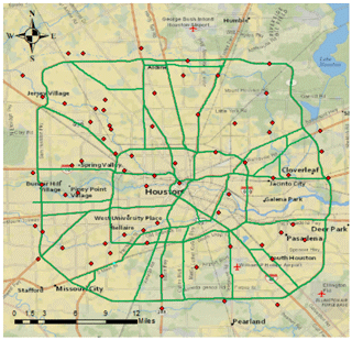
The study area is Houston, Texas, USA as shown in Fig. 1. In 2017, Hurricane Harvey made a landfall, causing USD 125 billion in economic loss, second only to Hurricane Katrina on record (NOAA, 2022). Major hospitals located in the northwest and southeast served as essential facilities for responding to the storm. For example, while searching for a missing family member during the storm, a patient sustained a head injury after a fall from his all-terrain vehicle. Emergency medical services (EMS) placed him in a cervical collar but were unable to reach LBJ, instead transferring him to a dump truck for transport (Chambers et al., 2020). Meanwhile, four major Interstate highways (IH 10, IH 610, IH 45, IH69) interlaced.

Figure 1 Main road network and sensor sites in Houston, TX.

2.2 Data

2.2.1 Data source

The rainfall data was retrieved from Harris County Flood Warning System (HCFWS, 2022), including daily rainfall values observed at 67 sensor sites and their coordinates. The road closure data was provided by the Texas Department of Transportation (TxDOT), containing roadway names, starting and ending points, and closure period. The flood map from the Federal Emergency Management Agency (FEMA, 2022), divides the study area into 100 return-year, 500 return year flood prone zones and the other. It is based on local topography and rainfall-runoff Hydrologic Engineering Certer-River Analysis System model (National Research Council, 2009). Finally, the state highway network shapefile was obtained from Federal Highway Administration (FHWA, 2021), with 4377 road segments totalling 638 km in length.

In this study, rainfall is considered as the primary driver of road closure.

2.2.2 Pre-processing

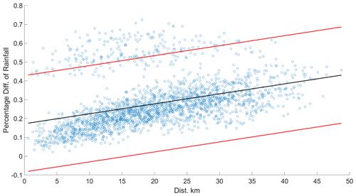
In a large quantity of rainfall data, some sensors behaved abnormally during Hurricane Harvey and were removed as outliers. Over the 5 d period from 25 to 29 August 2017, the average daily rainfall was most severe, between 3 inch and 12 inch. The sensors, which displayed a rainfall measurement of 0 due to data unavailability, were first eliminated. Furthermore, spatial analysis was performed to determine if additional outliers existed. In Fig. 2, each point represents the distance between a pair of sensors and the percentage difference in their recorded rainfall values. And the upper and lower bounds are plotted for the 95 % confidence interval for the linearly regressed line. Points outside the interval are considered as possible outliers and their relationship with nearby sensors are re-calculated. Those sensors outside of the interval are then removed. Finally, the rainfall data is obtained from 62 sensors. The training set contained the rainfall data and road closure data during 2017. The testing set covered the period from January to Augusts 2018.

Figure 2 Scatter plot of relationship between sensor distance and difference in rainfall.

Mandapaka et al. (2009) studied the correlation between rainfall and distance. The fitted curve, shown as Eq. (1), satisfies the exponential function, and the correlation decreases with the increase in distance. Thanks to the dense sensor network in the study area, the correlation between neighbouring sensors is high (i.e. 0.79–0.99).

$$\begin{array}{}\text{(1)}& y=\exp [-(x/\mathrm{40.15}{)}^{\mathrm{0.8}}]\end{array}$$

where x represents the distance between two sensor locations, and y represents the rainfall correlation.

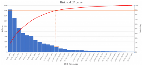
Moreover, relating the rainfall observed at sensors to the rainfall at road segments can be solved by spatial interpolation methods such as Kriging (Oliver and Webster, 1990). Figure 3 shows the percentage difference in segment-level rainfall derived from two methods: nearest sensor and Kriging method. The EP curve indicates that 90 % of these values are within 11 % in difference or less. The Kriging method is computationally intensive when applied to large datasets (e.g., daily rainfalls from 62 sensors). Furthermore, considering the numerous factors influencing rainfall within a very limited range makes the situation even more complex. The kriging method serves only as an approximate simulation approach. Thus, the method of nearest sensor is adopted hereafter.

Figure 3 Histogram & EP curve for rainfall percentage difference based on nearest sensor and Kriging method.

2.3 Logistic Regression Model

The equation of Logistic regression is shown as Eq. (2).

$$\begin{array}{}\text{(2)}& P\left(Y=\mathrm{1}|x\right)={\displaystyle \frac{\mathrm{1}}{\mathrm{1}+e^{-({\mathit{\omega }}^{T}x+b)}}}\end{array}$$

where Y=1 represents road closure, x represents the vector of multi-day rainfall, b represents the vector of constant and ω represents the matrix of weight for each independent variable. In Lee and Kim's (2021) study, 3–24 h rainfall data was used to predict road closures, excluding hysteresis effects. In contrast, this paper employs multi-day rainfall data to examine the role of lag effect.

The logarithmic probability of output Y=1 is a model expressed by the function of input x. The closer the value of b+ω^Tx is to positive infinity, the closer the probability value of $P\left(Y=\mathrm{1}|x\right)$ is to 1. In this paper, the cutoff value of p is set at 0.5. There are 2 models formulated as follow:

• Model I: One logistic regression model for the whole road network.

• Model II: Three different logistic regression model for three different flood prone zones respectively.

3 Results

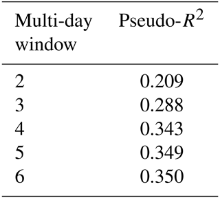
Table 1 shows the models using rainfall data over multiple windows and their Pseudo-R² value. Once the number of days reaches 4, the computational demand would increase rapidly for each additional day, but the improvement in the Pseudo-R² value become minimal. Therefore, the window of 4 d is selected.

Table 1 Model performance using rainfall data over multiple days.

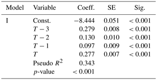
The result from Model I is summarized in Table 2. The overall model is significant, with p<.001 and R²=0.343. Meanwhile, all independent variables are significant at p<.001. T represents the current day and T-i represents the i day before it. While rainfall correlates positively to road closure, the influence of 3 d before the current day (T−3) and the current day (T) are much larger.

Table 2 Logistic regression for Model I (Sample size N=1 584 474).

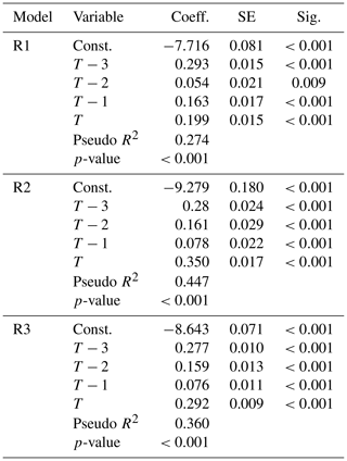
In Table 3 results from Model II are organized by different flood prone zones. R1 represents 100-year return-year zone, R2 represents 500-year return-year zone, and R3 represents the other. All independent variables are significant. Similarly, the coefficients for the 3 d prior and the current day are larger than others. In other word, the risk of road closure would be high when these two days experience heavy rainfall.

Table 3 Logistic regression for Model II (different return year with sample size N=1 584 474).

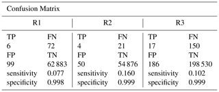
Since the excessive rainfall (and inducted road closure) is a relatively rare phenomena, the threshold of probability for predicting road closure is set to 0.1. The confusion matrix for Model II is shown in Table 4, where TP, FN, FP, and TN represent true positive, false negative, false positive, and true negative respectively. The numbers of case are given inside parentheses.

Table 4 Confusion matrix for validation.

According to Eqs. (2)–(4), the sensitivity of R1 model is 0.077, indicating that this model performs poorly on predicting road closure (Type I error). At the same time, the model is superior when predicting non road closure (with the specificity =0.999). The overall utility of the model would depend on traveller's detour cost. The model is more appropriate in scenarios where detour cost is low and more alternative routes are available.

$$\begin{array}{}\text{(3)}& {\displaystyle }\text{Sensitivity}={\displaystyle \frac{\text{TP}}{\text{TP}+\text{FN}}}\text{(4)}& {\displaystyle }\text{Specificity}={\displaystyle \frac{\text{TN}}{\text{TN}+\text{FP}}}\text{(5)}& {\displaystyle }\text{Accuracy}={\displaystyle \frac{\text{TN}+\text{TP}}{\text{TN}+\text{TP}+\text{FN}+\text{FP}}}\end{array}$$

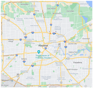
The closure probability at the road segment level can be aggregated to estimate accessibility to essential facilities during disasters. Here is an application to demonstrate the practical use of this model. An illustration is given for Harris Health Lyndon B. Johnson Hospital (labelled as Point 1 in Fig. 4) from two intersections (labelled as Points 2 and 3): Route 1: 1→2, Route 2: 3→1. Overlaid with rainfall data during Hurricane Harvey (26 to 29 August 2017), the probability of inaccessibility for Route 1 due to road closure is 81.5 %, and the probability for Route 2 is 99.2 %. Pre-storm preparations could have allowed for smoother and safer ride-out functioning for both hospital personnel and patients (Chambers et al., 2020).

Figure 4 Location of study hospital and the access from two intersections.

4 Modified model based on watershed

The national scope of FEMA flood maps, while providing a broad overview, can potentially overlook the unique attributes and varying hydrological dynamics that are intrinsic to specific regions.

Each area, due to its distinct topography and climate factors, can exhibit unique flood characteristics. These differences can significantly affect the nature and scale of flood risks, and thereby the effectiveness of mitigation measures. Therefore, it becomes imperative to adopt a more localized approach, requiring finer regional segmentation, which can more accurately capture the geo-difference of flood risks.

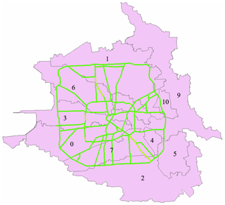
The HCFWS has provided a watershed division methodology, leveraging Geographic Information System (GIS) technology. The analysis encompasses various steps that involve utilizing GIS functions, such as Fill, Flow Direction, Flow Accumulation, Con, Stream Link, Stream Order, Stream To Feature, New Feature Class, Snap Pour Point, Watershed, and Raster to Polygon, to accurately delineate watersheds, determine flow paths, classify streams, convert data formats, and analyze hydrological patterns, enabling effective flood risk management and improved understanding of local hydrology. The conceptual representation of this GIS-based watershed division methodology is depicted in Fig. 5.

Figure 5 Watershed Division Map as Generated by the HCFWS (from HCFCDGISADMIN).

The numerals within the map correspond to the unique codenames assigned to each region, while the green lines delineate the transportation networks. However, those boundaries are based only on surface topography, and adjustments are then required to account for storm sewer systems that influence flow patterns. That adjustment is done manually based on review of storm sewer data.

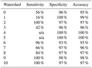
In a similar way to the previous methodologies, the modified model employs the logistic regression method as its analytical framework. This model utilizes daily precipitation data for Harris County from August 2017 as its independent variable. The dependent variable in this model is the operational status of roads within the area, defined as a binary outcome: whether the road is closed due to flooding or remains open. The model's data set was strategically partitioned into a training set and a test set. The training set, which comprises 75 % of the total data, was utilized to calibrate the logistic regression model. Conversely, the remaining 25 % of the data was retained as a test set, used to validate the model's predictive capacity and gauge its overall performance. The predictive outcomes of the testing set generated by the model are shown in Table 5.

Table 5 Logistic regression for Modified Model. n/a – not applicable.

In the context of this analysis, the sensitivity metrics for Area 4 and Area 5 are indicated as “n/a”, signifying “Not Applicable”. There are two plausible explanations. Firstly, these regions may inherently possess a higher resilience to flood events, attributable to various factors such as topography, built environment characteristics, and effective flood mitigation measures. This superior resilience could explain the absence of road closures during the extreme weather event. Secondly, the limited number of road segments under investigation within these two areas could have contributed to the observed outcomes. With a smaller dataset, the potential for statistical bias is amplified, possibly leading to skewed results.

Due to the data presented in Table 5, it can be observed that the specificity and accuracy measures remain relatively consistent with prior outcomes, demonstrating remarkable levels of precision. However, A noticeable improvement in the overall sensitivity can be seen, indicating a substantial improvement in the model's true positive rate.

Further analysis is partitioned into three sections. The first part consists of Area 1, exhibiting a persistently low sensitivity. Interpreted in practical terms, the likelihood of successfully predicting road closures in this area remains minimal. The expansive geographical area of Area 1, punctuated with complex terrain features, including existing river systems, might be accountable for this outcome. Consequently, factors influencing road closures in this region extend beyond mere rainfall, complicating the prediction capabilities of a model relying on a single input variable.

The second part, comprising Areas 0, 3, and 7, demonstrates medium sensitivity levels. Given their geographical locations in the southwest region of the study area, it is plausible that additional variables, such as social vulnerability and resilience index, might contribute to the complexity of predicting road closures in this sector.

Lastly, Areas 2, 6, 8, 9, and 10 exhibit high sensitivity levels, mainly concentrated in the central and southeastern parts of the study area. This observation suggests a strong correlation between rainfall and road closures in these specific regions, reinforcing the relevance of rainfall as a primary input variable in these contexts.

5 Conclusions

The rainfall values on 3 d prior and the current day contribute the most to the chance of road closure. This could be explained that the heavy rainfall at the beginning of a storm wash branches or woody debris onto roads and cause road closure. Such debris would also block drainage outlets, seriously reducing drainage capacity of the road (Flanagan et al., 1998). Current-day rainfall adds direct and immediate effect to exceeds drainage capacity (Hammami et al., 2019). An alternative interpretation of the time lag might consider its application within a specific temporal window, in line with the water's travel time within the study area. In addition, there are issues related to the regional division of the research. The modified model demonstrated markedly better results, indicating that establishing how to create a cluster is also crucial.

The results reveal two limitations that the predictions consistently lean towards no closure. This bias arises for two main reasons. First, the data collected is unbalanced, thus future research should strive to balance the data as much as possible during the pre-processing stage. Besides, in examining lag effects, both soil moisture and the generation of differential flows exert influence and thus must be taken into account.

For future study, distance to rivers, social vulnerability, and representation of drainage network could be added to the model to improve its sensitivity and overall performance. According to the regional analysis in this paper, flood risk analysis for personal preventative measures, emergency evacuations, or flood insurance policies, shouldn't be uniformly implemented across broad regions. Instead, they should be customized according to the local features, taking into account the unique socioeconomic traits of individual households and communities (Koks et al., 2015).