the Creative Commons Attribution 4.0 License.
the Creative Commons Attribution 4.0 License.
 | 19 Apr 2024
A tale of two floods: Hawkesbury-Nepean valley floods of February 2020 and March 2021
Katayoon Bahramian
Kesav Unnithan
Christoph Rüdiger
Jiawei Hou
Christopher Pickett-Heaps
Elisabetta Carrara
The Hawkesbury-Nepean valley is one of the largest coastal basins in NSW. It supports the local agriculture industry and is an important environmental asset. Due to its narrow sandstone gorges, which create natural choke points, floodwaters from its major tributaries can rapidly back up, rise and spill out onto the flood plain. Thus, the valley is flood-prone, with a history of disastrous events, aggravated by a constrained road network for evacuation.
Two flood events occurred in the Hawkesbury-Nepean valley in 2020 and 2021, however, the impact of each of those events was different in terms of lives lost (2 fatalities compared to none) and economic losses (more than AUD 2 billion compared to less than AUD 1 billion). In this study, reasons for the variation in impacts are explored by determining an inundation likelihood map, derived using a combination of the height above nearest drainage method and streamflow forecasts, and considering antecedent hydrological and climate conditions.
- Article
(8209 KB) - Full-text XML
- BibTeX
- EndNote


Floods along the eastern coast of Australia have always featured in Australia's natural hazard profile since records began, due to the presence of intra-annual or seasonal as well as interannual climate drivers which drive flood weather conditions in that area. These climate drivers are projected to be exacerbated by climate change, where heavy rainfall events are projected to increase in the East Coast region (National Hydrological Projections, East Coast Assessment Report 2022; Matic et al., 2022), changing the severity and frequency of floods, which will negatively impact socio-economic and ecosystem resilience.
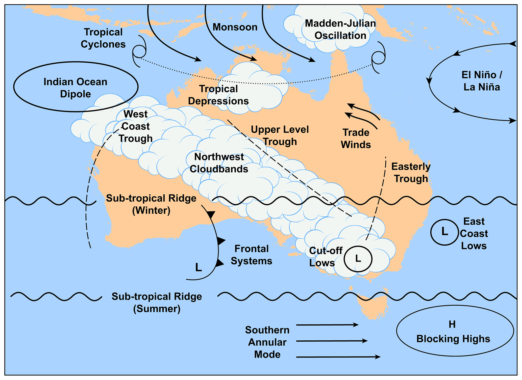
Figure 1Major climate drivers for flood weather (Source: © Bureau of Meteorology, 2010).
The intra-annual or seasonal drivers, shown in Fig. 1, include:
-
East coast lows (ECLs), which are intense low-pressure systems that occur on average several times each year off the eastern coast of Australia. ECLs will often rapidly intensify overnight making them one of the more dangerous weather systems, where individual east coast lows usually last for a few days. ECLs are most common during autumn and winter with a maximum frequency in June (Kiem et al., 2016).
-
Tropical cyclone seasons (TCS). The TCS officially runs November–April, but often TC activity is variable throughout the season. Storm surges accompanying TCs can exacerbate riverine flooding along the coast, where storm surges often accompany TCs (Needham et al., 2015).
-
Monsoon seasons (MS). MS is associated with cloudy conditions, lengthy periods of heavy rain, occasional thunderstorms and strong winds, often causing flooding. In addition, the Madden-Julian Oscillation can influence the timing and intensity of “active” monsoon periods in northern Australia, leading to enhanced rainfall – both in intensity and duration (Wheeler et al., 2009).
The interannual drivers, shown in Fig. 1, include:
-
La Niña conditions. There is an established relationship between La Niña strength and rainfall, where the greater the sea surface temperature and Southern Oscillation Index (SOI) difference from normal, the larger the rainfall response (Power and Callaghan, 2016). For example, the six wettest winter–spring periods on record for eastern Australia occurred during La Niña years, and there have been more TCs in the Australia region, with twice as many making landfall (Alexander and Hayman, 2008). La Niña conditions result in an increased likelihood of flooding.
-
A negative Indian Ocean Dipole (IOD). A negative IOD often results in more rainfall than average over south-eastern Australia. In conjunction with La Niña conditions, rainfall is above average over large parts of Australia. For example, during 2010, under La Niña conditions, a negative IOD developed, and combined to produce heavy rainfall and widespread flooding across eastern Australia (Lim and Hendon, 2017).
-
Landscape antecedent conditions. Wet antecedent conditions or saturated soil and full water stores can increase the flood maxima generated from an event such as heavy rainfall, TC or storm surge (Wasko et al., 2020).
The Hawkesbury-Nepean valley located along the southeast coast of New South Wales (NSW), is one of the largest coastal basins in NSW (Fig. 2a and b). It supports the local agriculture industry and hence is an important environmental asset. Flood risk in this valley has been described as the highest in NSW, if not Australia (Infrastructure NSW, 2021). This risk arises from several exposure and vulnerability factors, including the large and growing population, a constrained road network which poses challenges for evacuation, and low levels of flood awareness (Infrastructure NSW, 2021). In addition, the Hawkesbury-Nepean valley's unique topography and river network are environmental factors exacerbating flood risk, due to the contribution of 5 major tributaries or “taps” flowing into 1 river system – the “drain” – which is constrained by narrow downstream gorges (Fig. 2c). Due to the narrow sandstone gorges, which create natural choke points, floodwaters from its major tributaries can rapidly back up, rise and spill out onto the flood plain. This causes floodwaters to back up across floodplains to considerable depths –known as the “bathtub” effect (Fig. 2c). Thus, the valley is flood-prone, with a history of disastrous events, with over 100 floods recorded from 1799 up until 2021 (Infrastructure NSW, 2021).
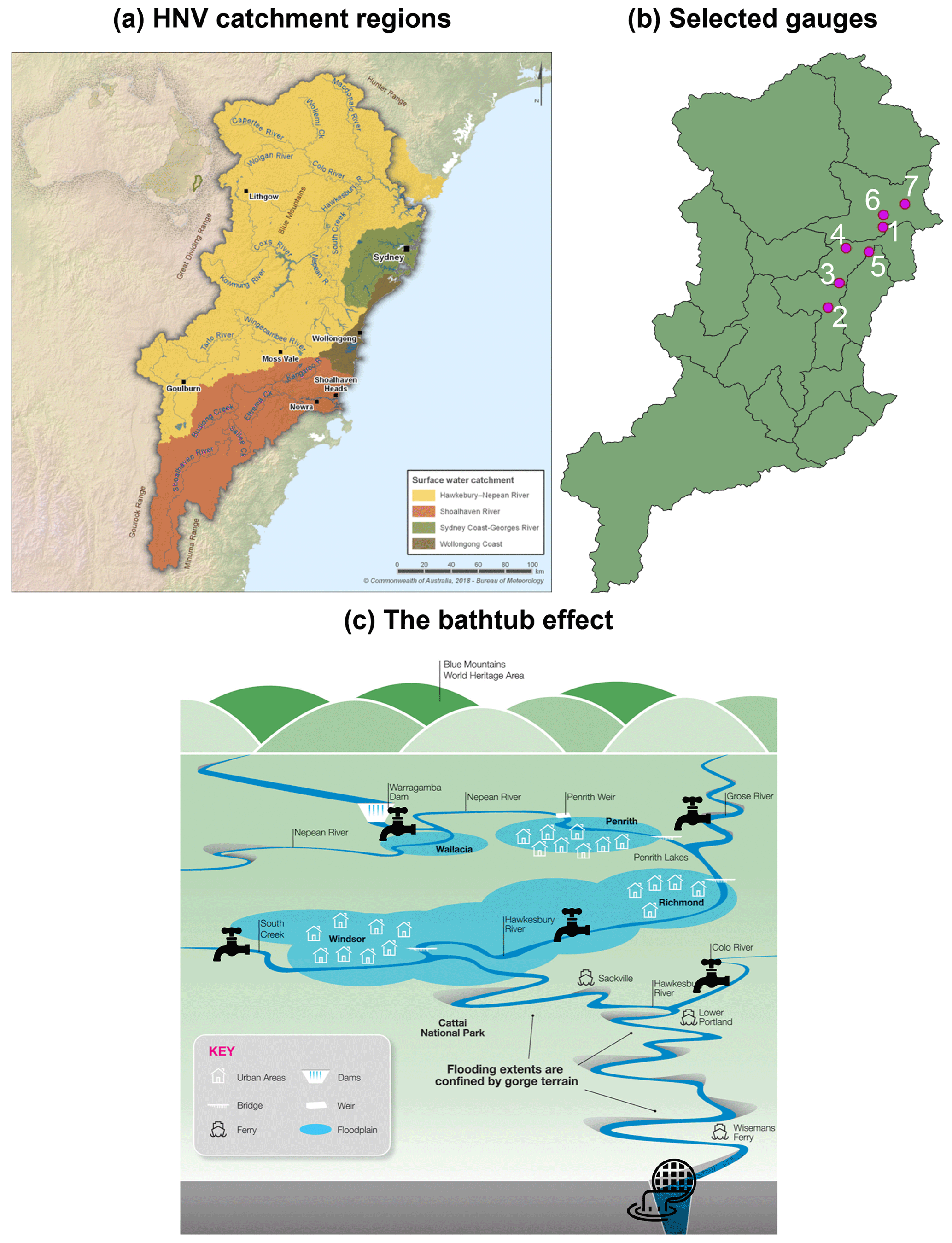
Figure 2(a) NSW catchment boundaries and rivers along the eastern coast, including the Hawkesbury-Nepean catchment in yellow. (b) Sub-catchment boundaries within the Hawkesbury-Nepean catchment and selected gauging stations: 1 – Sackville, 2 – Wallacia Weir, 3 – Penrith, 4 – North Richmond, 5 – Windsor PWD, 6 – Colo Junction and 7 – Webbs Creek. (c) Illustration of the “bathtub effect” with taps and drain, unique to the Hawkesbury-Nepean valley (adapted from Infrastructure NSW, 2021).
Two flood events occurred in the Hawkesbury-Nepean valley in 2020 and 2021, with near identical climate conditions, however, the impact of each of those events was different in terms of lives lost (2 fatalities compared to none) and economic losses (over two billion AUD compared to less than one billion AUD) (source: Infrastructure NSW, 2021; Insurance Council of Australia, 2021). In this study, the reasons for the variation in impacts are explored by determining:
- i.
the antecedent landscape conditions,
- ii.
the climatic conditions, and
- iii.
the inundation extent and depth,
for each event in order to gauge and compare the resultant hazard footprint.
This study employs the height above nearest drainage (HAND) methodology along with analysis of observational datasets (both grid and point based) to compare the two flood events.
2.1 Probabilistic inundation mapping methodology
The height above nearest drainage (HAND) approach to flood inundation mapping is a simple approach based on the height of the flood depth (Fig. 3a). The HAND methodological workflow can be described in the following steps:
-
The contributing catchment to a defined outlet is rasterized to the resolution of the supporting DEM.
-
Flow direction and accumulation in each grid cell is derived using a D8 algorithm (O'Callaghan and Mark, 1984).
-
In-stream and out-of-stream cells are identified using the flow line vector (river defined by the DEM).
-
The relief between all out-of-stream cells from their nearest in-stream cell is calculated to define a HAND raster.
-
From a given flow rate, a rating curve can be used to convert flow to water-level.
-
Subtracting the HAND raster from the water-level raster yields a water-level above-surface raster. All values greater than zero show the estimated flood height at each cell.
The height of the riverbank versus the height of the flood depth where the difference between each is taken as the volume of water spilling out into the flood plain (Fig. 3a).

Figure 3(a) HAND illustration for a given streambed. (b) The cell representation of the HAND workflow (adapted from Lababidi (2021)). (c) Illustration of the Geofabric toolset. (d) DEM of the Hawkesbury-Nepean valley Sackville (station 1) region in with sub-catchment boundaries in white (left panel) and zoomed in from orange box (right panel).
An illustration of this workflow is given in Fig. 3 top panel (b) (Lababidi, 2021). The probabilistic approach takes the HAND depth uncertainty into account and generates an ensemble based on the increments between the lower and upper 95th interval bounds, producing an ensemble of water-level above-surface rasters which are then turned into probabilities for each cell based on the number of times that cell is above zero. The HAND approach used in this study uses:
-
a varying Mannings roughness coefficient to estimate streamflow, as a function of hydraulic radius and reach slope (Marcus et al., 1992),
-
a HAND threshold position of 0.25 m (in order to calculate a HAND raster; Unnithan et al., 2020),
-
uncertainty in bankfull geometry to calculate an ensemble of HAND rasters,
-
a 1D vector flow routing scheme (Yamazaki et al., 2011), and,
-
captures water management and backwater effects (explained in Sect. 2.2; Mizukami et al., 2016).
2.2 Capturing water management and backwater effects
Due to the unique “bathtub effect” in the Hawkesbury-Nepean catchment, it is important that backwater effects or upstream flooding caused by downstream conditions such as channel restriction and/or high flow in a downstream confluence stream are considered. In addition, given the large dam in this catchment, the dam outflows also need to be considered.
Backwater effects are incorporated into the HAND approach via the 1D flow routing scheme (Yamazaki et al., 2011; Mizukami et al., 2016). During a flood event, the dam storage is monitored and if the storage has not yet reached capacity, the upstream discharge contributions of the reach where the dam is located are set to be zero.
2.3 Data
The HAND methodology calls for a hydrologically conditioned digital elevation model (DEM) and gridded runoff or streamflow data. The DEM used was the Bureau of Meteorology's Geofabric (Fig. 3c and d) which is a national dataset based on mapped hydrological features and a 1 s digital elevation model (DEM). Geofabric v3 (Bureau of Meteorology Water Information Services, 2015) contains the following products used in this study:
-
Geofabric Surface Network: Network representation of hydrological features, including over 2.5 million stream segments and 6000 gauging stations.
-
Geofabric Surface Catchments: Catchment boundaries derived from a 1 s Digital Elevation Model, with approximately 7 million base level catchments.
The gridded runoff data used is hydrological simulation data from the Bureau of Meteorology's operational landscape model, AWRA-L v7 (https://www.awo.bom.gov.au, last access: 18 October 2023, Frost et al., 2021). It simulates the flow of water through the landscape with precipitation entering the grid cell through vegetation and soil moisture stores and then out of the grid cell as evapotranspiration, runoff or deep drainage to the groundwater. Thus, runoff generated via AWRA-L considers antecedent conditions.
All datasets used in the analysis are:
-
the Australian Water Availability Project rainfall data (Bureau of Meteorology AWAP, 2022),
-
the AWRA-L v7 root zone soil moisture data (Frost et al., 2021),
-
the Bureau of Meteorology streamflow gauging station data for a selection of “high impact” locations (Bureau of Meteorology Flood Warning Services, 2022),
-
the global bankfull width and depth database (Andreadis et al., 2013).
In this section we compare flood characteristics, catchment antecedent conditions, climatic conditions, and hazard footprints between the two flood events.
3.1 Comparison of flood characteristics
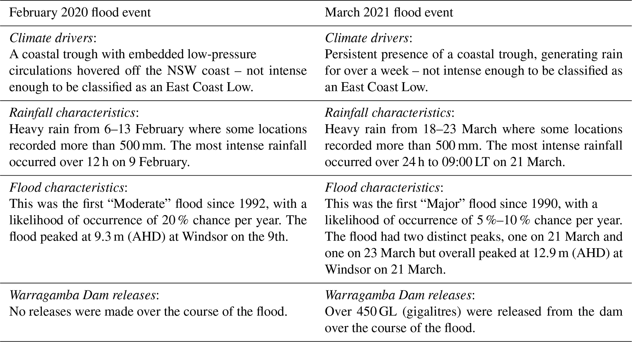
A comparison between the two flood events in the Hawkesbury-Nepean valley; detailing rainfall, climate drivers, and flood characteristics are described in Table 1. Flood characteristics are described by a classification system used by Australia's emergency services as well as a chance of occurrence which is expressed as a likelihood of a flood of a certain classification occurring in a given year. Floods are classified via a three-tiered scheme: “Minor”, “Moderate” and “Major” where the classification levels at each station are decided by the jurisdictions and are based on water levels which cause certain impacts.
Table 1Flood event characteristics for the February 2020 and March 2021 floods in the Hawkesbury-Nepean valley (Infrastructure NSW, 2021).
3.2 Comparison of antecedent conditions
The February 2020 floods came off the back of the notorious “Black Summer”, a period of which, due to its intensity, size, duration, and uncontrollability, was considered a megafire (Geary et al., 2022). Black Summer occurred due to an extended period of El Niño events, causing a prolonged period of drought and very dry landscape conditions (Squire et al., 2021). This can be seen in Fig. 4 where the root zone soil moisture (from AWRA-L v7) in the Hawkesbury-Nepean catchment is mostly between – and 0 and 0.3 fraction fullness (Fig. 4a, rootzone soil moisture plot) and the Warragamba Dam (which services the Hawkesbury-Nepean catchment) storage is at ∼40 % or ∼1000 GL (Fig. 4c and d, bar charts, panels, Water NSW). In comparison, the March 2021 floods occurred in a La Niña year, where soil moisture conditions were wet, hovering between 0.5 and 0.8 fraction fullness for most of the catchment (Fig. 4b, rootzone soil moisture plot) and the Warragamba Dam storage is at ∼90 % or ∼2500 GL (Fig. 4, bar chart; Water NSW, 2022).

Figure 4Antecedent conditions. (a) Soil moisture prior to February 2020 (c) Water storage in GL and percentage fullness of Warragamba dam prior to February 2020 and March 2021 event.
3.3 Comparison of rainfall
The rainfall totals and average daily rainfall over both events, calculated using the climate data from AWAP, are similar, particularly when comparing the average daily rainfall across both events (Fig. 5c and d). However, the February 2020 flood event rainfall totals and average daily rainfalls are slightly higher over the Hawkesbury-Nepean catchment (Fig. 5).
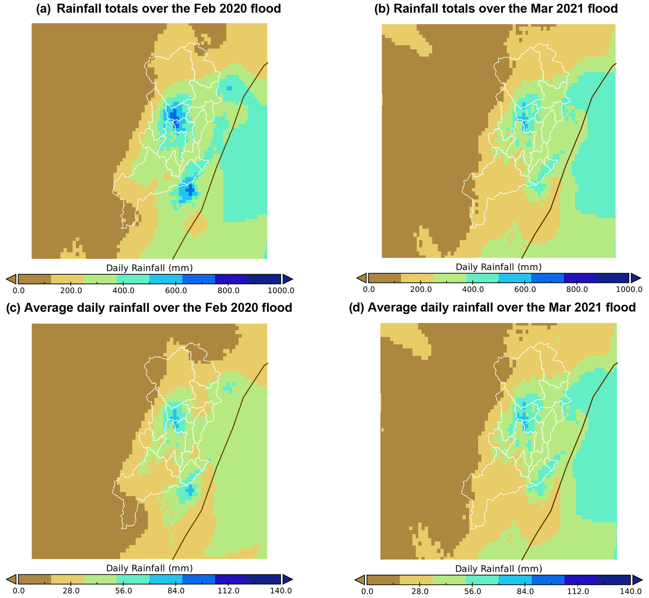
Figure 5Rainfall totals; summed over the flood events and daily averages. (a) Totals over the February 2020 flood, (b) Totals over the March 2021 flood. (c) Averaged daily totals for the February 2020 flood. (d) Averaged daily totals for the March 2021 flood.
3.4 Comparison of water levels
The resulting streamflow generated from both events can be extrapolated from water level plots or hydrographs shown in Fig. 6. These gauging stations are: 1 – Sackville, 2 – Wallacia Weir, 3 – Penrith, 4 – North Richmond, 5 – Windsor PWD, 6 – Colo Junction and 7 – Webbs Creek, considered to be “high impact” locations, where their locations are shown in Fig. 2b. The hydrographs from the 2021 event show that the excess streamflow generated is larger than for the 2020 event, where water level peaks are higher (except for Wallacia Weir) and the duration of the event is longer across the seven gauging stations. Even though the actual peak between events is very similar between events for station 2 (Wallacia Weir), due to the high concentration of rainfall in that region for the 2020 event (see Fig. 5a), however, given the longer duration of the March 2021 event, more water is flowing onto the flood plane comparatively. For individual stations, it is interesting to note that the peak of the hydrograph of station 6 (Colo Junction) in the February 2020 event arrives significantly earlier than the peaks for other stations, possibly due to the after effects of the bushfires on the land cover, as well as the timing of rainfall flowing into the Colo River region.
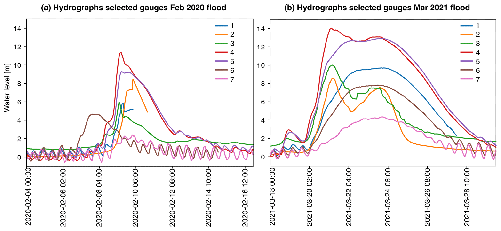
Figure 6Hydrographs for the 7 selected gauging stations for the February 2020 (a) and March 2021 (b) floods in Hawkesbury-Nepean valley. Gaps in the data are due to the cessation of monitoring when flood levels decrease to back below minor.
3.5 Comparison of flood extent and depth
Probabilistic inundation extents and depths (where depth is calculated relative to the bankfull elevation) are produced via the aforementioned methodology (Sect. 2) for the Sackville region of the Hawkesbury River (validation shown in Appendix A). Both the depth and probability of inundation for the 2021 event are higher (darker colors) than for the 2020 event and the inundation extent covers a larger area for the 2021 event, as expected from the flood classifications (“Moderate” in 2020 vs. “Major” in 2021).
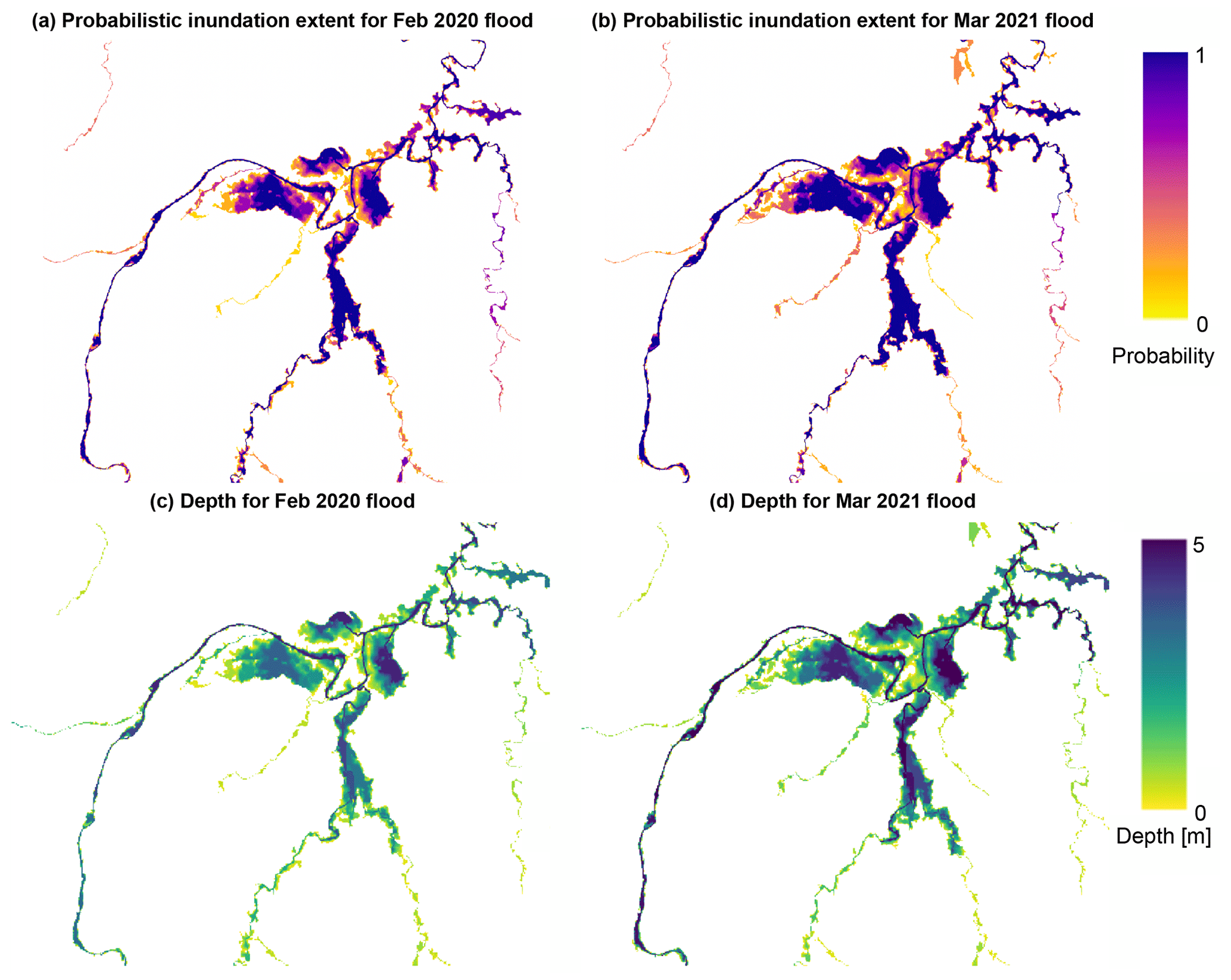
Figure 7Probabilistic inundation extents and depths. (a) Probabilistic inundation extent for the February 2020 flood. (b) Probabilistic inundation extent for the March 2021 flood. (c) Flood depth for the February 2020 flood. (d) Flood depth for the March 2021 flood.
The description of climate conditions and rainfall totals were remarkably similar between the two flood events; February 2020 and March 2021 (Table 1). In fact, the rainfall totals were slightly higher in certain regions during the February 2020 event (Fig. 5). Post event reviews have classified the February 2020 event as a 1 in 5 event, but the March 2021 event as a 1 in 20 event (Infrastructure NSW, 2021). This is also consistent with the inundation maps generated via the HAND technique (Fig. 7) where the depth and probability of inundation extent are larger for the 2021 flood event.
The impacts between the two events are outlined in Table 2. Table 2 shows that in comparison, the impacts of the March 2021 Flood Event are more severe in terms of affected areas, damages and fatalities. This tallies with the event classifications (Infrastructure NSW, 2021) as well as the HAND probabilistic inundation and depth maps (Fig. 7).
Table 2Flood impacts for the February 2020 and March 2021 floods in the Hawkesbury-Nepean valley (Infrastructure NSW, 2021; Insurance Council of Australia, 2021).

Upon examination of the antecedent soil moisture conditions, the dam storages and rainfall totals (Figs. 4 and 5), the major differences between the events are the antecedent soil moisture and dam storages. This is an important finding to note when considering that even though heavy rainfall events are projected to increase under climate change scenarios, the annual average rainfall is projected to decrease in NSW (Matic et al., 2022). This means that soil moisture conditions may be drier and affect flood maxima in much the same way as for the February 2020 flood event. Several studies examining the relationship between flood maxima and antecedent catchment conditions also agree with this study's findings – dry catchment conditions decrease flood maxima and conversely wet catchment conditions increase flood maxima (Sharma et al., 2018; Wasko et al., 2020). Thus, future work examining projected flooding in the Hawkesbury-Nepean catchment would need to also consider dam outflows and catchment antecedent conditions – a whole water cycle approach, rather than solely projecting climate fields.
The limitations of this study include the assumptions and shortcomings of the implementation of the HAND methodology employed, where according to our validation (see Appendix A), the number of cells inundated is overestimated. Further tuning would be enhanced by using additional events in the same region. In addition, the HAND methodology could be improved by:
-
Further hydrological conditioning of the DEM plus blending with LiDAR.
-
Routing the gridded runoff before ingesting.
-
Using a more sophisticated routing and backwater scheme.
There are many more fields we could have studied in terms of antecedent conditions and flood characteristics, however the soil moisture, dam storage, hydrographs from gauging stations at high impact locations, and rainfall totals told the full story.
Two flood events occurred in the Hawkesbury-Nepean valley in 2020 and 2021, with near identical climate conditions and thus rainfall patterns, however, the impacts from these events were classed as 1 in 5 and 1 in 20 events respectively; where the 2021 event resulted in 2 more lives lost, above AUD 1 billion more in damages and approximately 10 times more insurance claims. This study found that the antecedent catchment conditions prior to the flood events played a significant role in limiting the hazard footprint depth and extent of the February 2020 event, and thus its impact. Where drier conditions led to no dam outflows, filling of soil moisture and ground water storage deficits, which in turn led to less excess streamflow generated, and therefore less area inundated across the catchment.
The validity of the HAND results over both events is examined by comparison with Sentinel 2 data across the Sackville area of the catchment, on 10 February 2020 and 23 March 2021. The metrics used for validation are the: Critical Success Index (CSI), Youden's Index (YI), and Cohens Kappa (CK). The three metrics were used to get a more holistic measure of performance where CSI penalizes false positives in comparison to the other metrics (Fig. A1 top panels), YI is the likelihood of an inundated cell in the model in cells that are inundated versus those that are not inundated in the observations, and CK is a statistic that is used to measure inter-rater reliability (and intra-rater reliability) for qualitative (categorical) items (Schaefer, 1990; Fluss et al., 2005; Ben-David, 2008). The stringent validation metrics show the HAND methodology is performant, with most metrics greater than 0.5 in value across both events. It does however show that the HAND methodology employed in this study tends to overestimate the number of inundated cells.
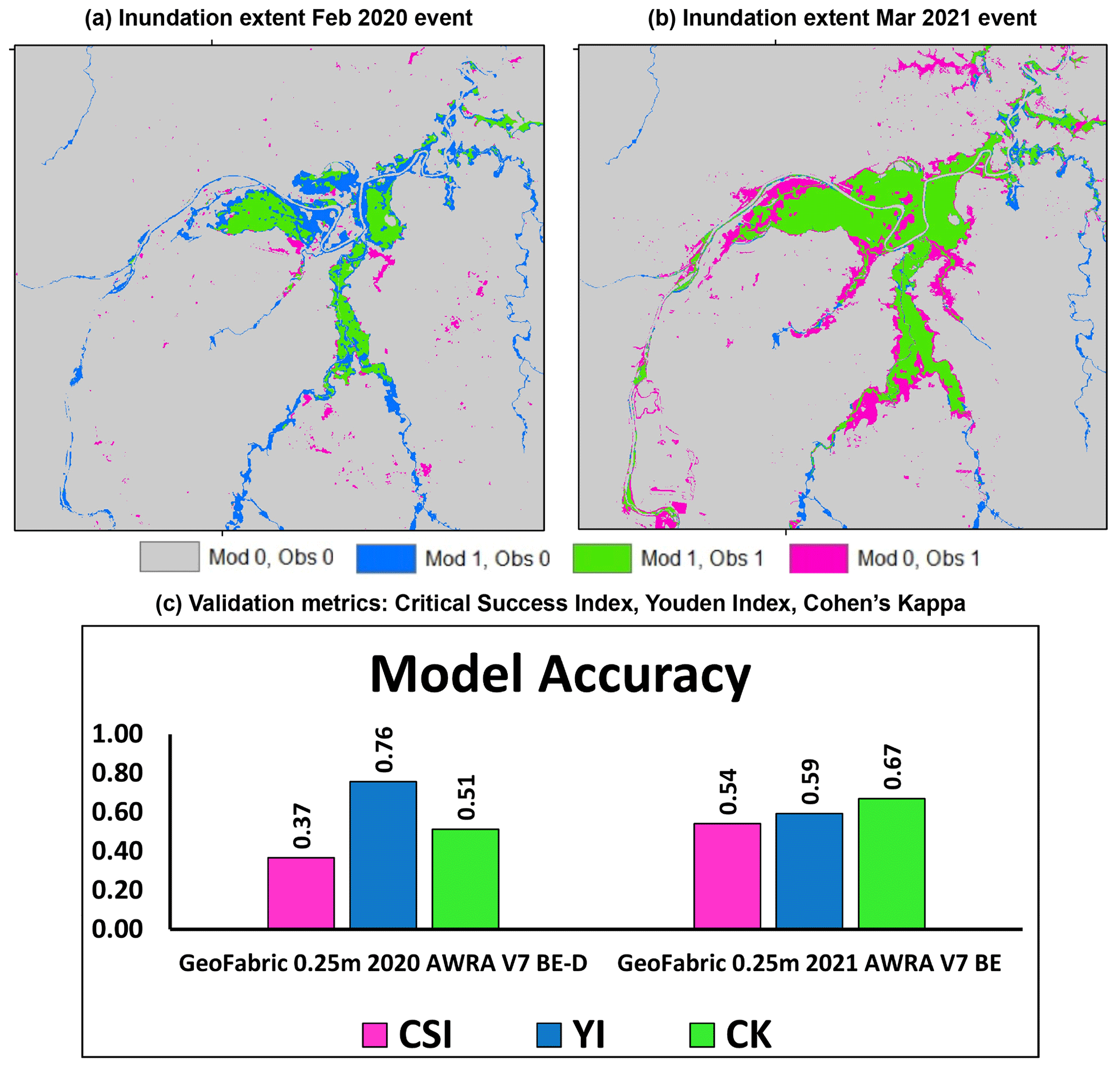
Figure A1Flood event validation for the February 2020 and March 2021 floods in Hawkesbury-Nepean valley. (a) Spatial plot of CSI validation for the February 2020 flood. (b) Spatial plot of CSI validation for the March 2021 flood. (c) All validation metrics calculated over the validation area presented in a bar chart.
Data and software available on request depending on licensing agreements.
WS: Conceptualization, Methodology, Formal analysis, Writing – original draft, Visualization. KB: Conceptualization, Methodology, Writing – review & editing. KU: Conceptualization, Investigation, Software, Methodology. CR: Conceptualization, Investigation, Methodology. JH: Methodology, Writing – review & editing. CPH: Writing – review & editing. EC: Conceptualization, Funding acquisition.
The contact author has declared that none of the authors has any competing interests.
Publisher's note: Copernicus Publications remains neutral with regard to jurisdictional claims made in the text, published maps, institutional affiliations, or any other geographical representation in this paper. While Copernicus Publications makes every effort to include appropriate place names, the final responsibility lies with the authors.
This article is part of the special issue “ICFM9 – River Basin Disaster Resilience and Sustainability by All”. It is a result of The 9th International Conference on Flood Management, Tsukuba, Japan, 18–22 February 2023.
This work was funded by the Australian Climate Service. The Australian Climate Service provides improved information, data, intelligence and expert advice on climate risks and impacts to support and inform decision-making. The Australian Climate Service is a partnership between the Bureau of Meteorology, CSIRO, the Australian Bureau of Statistics, Geoscience Australia. The authors would like to acknowledge the reviewers who greatly improved this paper. The authors would also like to acknowledge the support given by the Australian Bureau of Meteorology, in particular, the Hydrology Science section.
This research has been supported by the Australian Climate Service.
This paper was edited by Mamoru Miyamoto and reviewed by two anonymous referees.
Alexander, B. and Hayman, P.: The Regional Institute – Can we use forecasts of El Nino and La Nina for frost management in the Eastern and Southern grains belt?, ASA 2008 14th AAC, http://www.regional.org.au/au/asa/2008/concurrent/farming-uncertain-climate/5623_alexanderbm.htm (last access: 18 October 2023), 2008. a
Andreadis, K. M., Schumann, G. J.-P., and Pavelsky, T.: A simple global river bankfull width and depth database, Water Resour. Res., 49, 7164–7168, https://doi.org/10.1002/wrcr.20440, 2013. a
Ben-David, A.: About the relationship between ROC curves and Cohen's kappa, Eng. Appl. Artif. Intel., 21, 874–882, https://doi.org/10.1016/j.engappai.2007.09.009, 2008. a
Bureau of Meteorology: Australia's Climate Drivers, http://www.bom.gov.au/climate/about/ (last access: 1 January 2010), 2010. a
Bureau of Meteorology AWAP: Australian Gridded Climate Data (AGCD)/AWAP, v1.0.0 Snapshot (1900-01-01 to 2022-12-31), Bureau Data Catalogue, http://www.bom.gov.au/metadata/catalogue/19115/ANZCW0503900567 (last access: 18 October 2023), 2022. a
Bureau of Meteorology Flood Warning Services: Flood Warning Services, National flood forecasting and warning service, Water Information, Bureau of Meteorology, http://www.bom.gov.au/water/floods/floodWarningServices.shtml (last access: 18 October 2023), 2022. a
Bureau of Meteorology Water Information Services: Australian Hydrological Geospatial Fabric|Bureau Data Catalogue, http://www.bom.gov.au/water/geofabric/ (last access: 18 October 2023), 2015. a
Fluss, R., Faraggi, D., and Reiser, B.: Estimation of the Youden Index and its associated cutoff point, Biometr. J., 47, 458–472, https://doi.org/10.1002/bimj.200410135, 2005. a
Frost, A. J., Ramchurn, A., and Smith, A.: The Australian Landscape Water Balance model (AWRA-L v7) Technical Description of the Australian Water Resources Assessment Landscape model version 7, https://awo.bom.gov.au/assets/notes/publications/ (last access: 18 October 2023), 2021. a, b
Geary, W. L., Buchan, A., Allen, T., Attard, D., Bruce, M. J., Collins, L., Ecker, T. E., Fairman, T. A., Hollings, T., Loeffler, E., Muscatello, A., Parkes, D., Thomson, J., White, M., and Kelly, E.: Responding to the biodiversity impacts of a megafire: A case study from south‐eastern Australia's Black Summer, Divers. Distrib., 28, 463–478, https://doi.org/10.1111/ddi.13292, 2022. a
Infrastructure NSW: Hawkesbury-Nepean River March 2021 Flood Review – Final Report, © Infrastructure NSW, https://www.infrastructure.nsw.gov.au/media/3315/hnr-march-2021-flood-review.pdf (last access: 18 October 2023), 2021. a, b, c, d, e, f, g, h, i
Insurance Council of Australia: Annual report/Insurance Council of Australia Limited, https://insurancecouncil.com.au/ (last access: 18 October 2023), 2021. a, b
Kiem, A. S., Twomey, C., Lockart, N., Willgoose, G., Kuczera, G., Chowdhury, A. F., Manage, N. P., and Zhang, L.: Links between East Coast Lows and the spatial and temporal variability of rainfall along the eastern seaboard of Australia, J. South. Hemisph. Earth Syst. Sci., 66, 162–176, https://doi.org/10.22499/3.6602.006, 2016. a
Lababidi, S.: An evaluation of the Height Above Nearest Drainage (HAND) flood mapping methodology with the implementation of multivariant linear regression algorithm, Northeaster University, https://doi.org/10.17760/D20409241, 2021. a, b
Lim, E. P. and Hendon, H. H.: Causes and Predictability of the Negative Indian Ocean Dipole and Its Impact on la Niña during 2016, Sci. Rep., 7, 1–11, https://doi.org/10.1038/s41598-017-12674-z, 2017. a
Marcus, W. A., Roberts, K., Harvey, L., and Tackman, G.: An evaluation of methods for estimating Manning's n in small mountain streams, Mount. Res. Dev., 12, 227–239, https://doi.org/10.2307/3673667, 1992. a
Matic, V., Bende-Michl, U., Hope, P., Srikanthan, S., Oke, A., Khan, Z., Thomas, S., Sharples, W., Kociuba, G., Peter, J., Vogel, E., Wilson, L., and Turner, M.: East Coast – National Hydrological Projections Assessment report, https://awo.bom.gov.au/assets/notes/publications/ (last access: 18 October 2023), 2022. a, b
Mizukami, N., Clark, M. P., Sampson, K., Nijssen, B., Mao, Y., McMillan, H., Viger, R. J., Markstrom, S. L., Hay, L. E., Woods, R., Arnold, J. R., and Brekke, L. D.: MizuRoute version 1: A river network routing tool for a continental domain water resources applications, Geosci. Model Dev., 9, 2223—2228, https://doi.org/10.5194/gmd-9-2223-2016, 2016. a, b
Needham, H. F., Keim, B. D., and Sathiaraj, D.: A review of tropical cyclone-generated storm surges: Global data sources, observations, and impacts, Rev. Geophys., 53, 545–591, https://doi.org/10.1002/2014RG000477, 2015. a
O'Callaghan, J. F. and Mark, D. M.: The extraction of drainage networks from digital elevation data, Comput. Vis. Graph. Image Process., 28, 323–344, https://doi.org/10.1016/S0734-189X(84)80011-0, 1984. a
Power, S. B. and Callaghan, J.: The frequency of major flooding in coastal southeast Australia has significantly increased since the late 19th century, J. South. Hemisp. Earth Syst. Sci., 66, 2–11, https://doi.org/10.1071/es16002, 2016. a
Schaefer, J. T.: The Critical Success Index as an Indicator of Warning Skill, Weather Forecast., 5, 570–575, https://doi.org/10.1175/1520-0434(1990)005<0570:tcsiaa>2.0.co;2, 1990. a
Sharma, A., Wasko, C., and Lettenmaier, D. P.: If Precipitation Extremes Are Increasing, Why Aren't Floods?, Water Resour. Res., 54, 8545–8551, https://doi.org/10.1029/2018WR023749, 2018. a
Squire, D. T., Richardson, D., Risbey, J. S., Black, A. S., Kitsios, V., Matear, R. J., Monselesan, D., Moore, T. S., and Tozer, C. R.: Likelihood of unprecedented drought and fire weather during Australia's 2019 megafires, npj Clim. Atmos. Sci., 4, 64, https://doi.org/10.1038/s41612-021-00220-8, 2021. a
Unnithan, S. L., Biswal, B., and Rüdiger, C.: Flood inundation mapping by combining GNSS-R signals with topographical information, Remote Sens., 12, 3026, https://doi.org/10.3390/RS12183026, 2020. a
Wasko, C., Nathan, R., and Peel, M. C.: Changes in Antecedent Soil Moisture Modulate Flood Seasonality in a Changing Climate, Water Resour. Res., 56, e2019WR026300, https://doi.org/10.1029/2019WR026300, 2020. a, b
Water NSW: Greater Sydney Dam Levels – WaterNSW, https://www.waternsw.com.au/nsw-dams/nsw-storage-levels/greater-sydney-dam-levels (last access: 18 October 2023), 2022. a, b
Wheeler, M. C., Hendon, H. H., Cleland, S., Meinke, H., and Donald, A.: Impacts of the Madden-Julian oscillation on australian rainfall and circulation, J. Climate, 22, 1482–1498, https://doi.org/10.1175/2008JCLI2595.1, 2009. a
Yamazaki, D., Kanae, S., Kim, H., and Oki, T.: A physically based description of floodplain inundation dynamics in a global river routing model, Water Resour. Res., 47, W04501, https://doi.org/10.1029/2010WR009726, 2011. a, b