the Creative Commons Attribution 4.0 License.
the Creative Commons Attribution 4.0 License.
 | 19 Apr 2024
Methods to create hazard maps for flood disasters with sediment and driftwood
Daisuke Harada
Shinji Egashira
As flood disasters with sediment and driftwood are becoming severe, it is required to evaluate the risk of such disasters. The present study proposes methods to create hazard maps for such type of flood disasters using a watershed model and a 2-D flood flow model, and applied the methods to the Akatani river flood disaster in 2017 to discuss their applicability and challenges. The upstream boundary conditions of 2-D flood flow model are specified for the hydrographs of flow discharge, sediment discharge and driftwood discharge by using the results obtained from their basin model. As a result of the Akatani river simulation with the proposed methods, we found that the computational results reproduce the inundation area and elevation change, and the proposed methods are effective in creating flood hazard maps with sediment and driftwood.
- Article
(5182 KB) - Full-text XML
- BibTeX
- EndNote


When heavy rainfall occurs in mountainous areas, it causes landslides and debris flows at numerous locations in a watershed. The landslides and debris flows generate numerous amounts of sediment and large wood. Once these sediment and large wood are supplied to the river channel, they are transported downstream by the flood flow. In downstream areas, large wood accumulation takes place at many locations, such as bridges and sediment deposition areas and influences the flood flow. Recently, these types of flood hazards have been reported in numerous places over the world (e.g., Comiti et al., 2008; Harada and Egashira, 2018; Lucia et al., 2018).
To mitigate such flood disasters, it is necessary to predict possible hazard occurrences and develop hazard maps so that residents understand the possible hazards and evacuate appropriately. However, compared to flood hazard maps, there are not enough methods to assess and develop hazard maps for flood hazards with sediment and driftwood. To evaluate such flood hazards, it is necessary to obtain a time series of the water, sediment, and driftwood discharged from the watershed and to evaluate its effect on flood flows at downstream areas. Although several previous studies have attempted to evaluate such flood hazards (e.g., Liu et al., 2022; Huang et al., 2022), methods to evaluate flood hazards from the above perspective have not yet been established. This study proposes methods to create hazard maps for such types of flood disasters by combining a watershed model and a 2-D flood flow model, and applied the methods to the Akatani river flood disaster in 2017 to discuss their applicability and challenges.
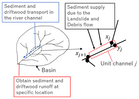
Figure 1Conceptual illustrations of a method for evaluating water, sediment and driftwood runoff from a basin.
2.1 Evaluation of water, sediment and driftwood runoff from a watershed
In this study, we propose an integrated method to simulate rainfall-runoff, landslide and debris flow, and sediment and driftwood transport in the river channel to obtain a time series of sediment and driftwood discharged from the watershed at an arbitrary location.
Figure 1 illustrates these processes conceptually. The occurrence of landslide, debris flow, and driftwood transport induced by a landslide on a hill slope are evaluated based on the method of Yamazaki and Egashira (2019). Slope stability analysis to evaluate the landslide occurrence is performed in the slope cell of the Rainfall-runoff-inundation (RRI) model developed by Samaya et al. (2012). The sediment transport that accompanies the landslide is analyzed using the equation of a mass system, from the point of origin to the location where the deposition occurs, and when the sediment reaches the river channel, it is treated as a sediment supply to the channel.
In the river channel, following the method proposed by Egashira and Matsuki (2000), a section that includes the upstream confluence (xj, yj) and excludes the downstream confluence point (xj+1) is designated as the unit channel, as shown in Fig. 1, and the sediment and large wood runoff for the entire basin is predicted by allocating the unit channels in series and parallel. This modeling allows for simple and stable analysis of sediment and large wood transport in complex channel networks. Therefore, the riverbed evolution in each unit channel is described as follows;
where zb is the bed elevation, λ is the sediemnt porosity, Bj and Lj are the width and length of the unit channel j, respectively; Qbi(xj) is the bedload transport rate for grain size di of the unit channel j; V is the sediment volume supplied from the slope; pVi is the content ratio in the sediment supplied from the slope for the grain size di, Ei and Di are the erosion and deposition rate of suspended sediment for grain size di.
To treat a large number of driftwood transport, we assume that the wood pieces behave as neutral buoyant particles, as this assumption allows the introduction of the convection equation (Harada and Egashira, 2018). In this method, we assume that the erosion and deposition of driftwood occurs in proportion to sediment erosion and deposition, based on the idea that when the sediment is deposited, the wood particles are also deposited on the riverbed, and when sediment is eroded, wood particles are also taken into the water. Also, assuming that large wood accumulation occurs at artificial structures such as bridges, the convection equation is coupled with the storage equation of driftwood in the channel bed.
In case of (Sediment deposition)
where cdrf is the driftwood concentration, h is the depth, Q(xj) is the flow discharge of the unit channel j, c∗ is the sediment concentration of the river bed, vn is the is the inward velocity normal to the structure such as the bridge, pb is the probability that large wood is captured at structures, ranging from 0 to 1 (we employ 1 in this study), Vdrf is the volume of driftwood supplied from the slope due to the debris flow. Function r(txy) is introduced to describe the phenomena that the driftwood erosion does not occur at depths shallower than a certain water depth, and large wood deposition does not occur at depths deeper than a certain water depth. Due to space limitation, please refer to Harada and Egashira (2018) for specific functions r(txy) and treatment for the sediment erosion case.
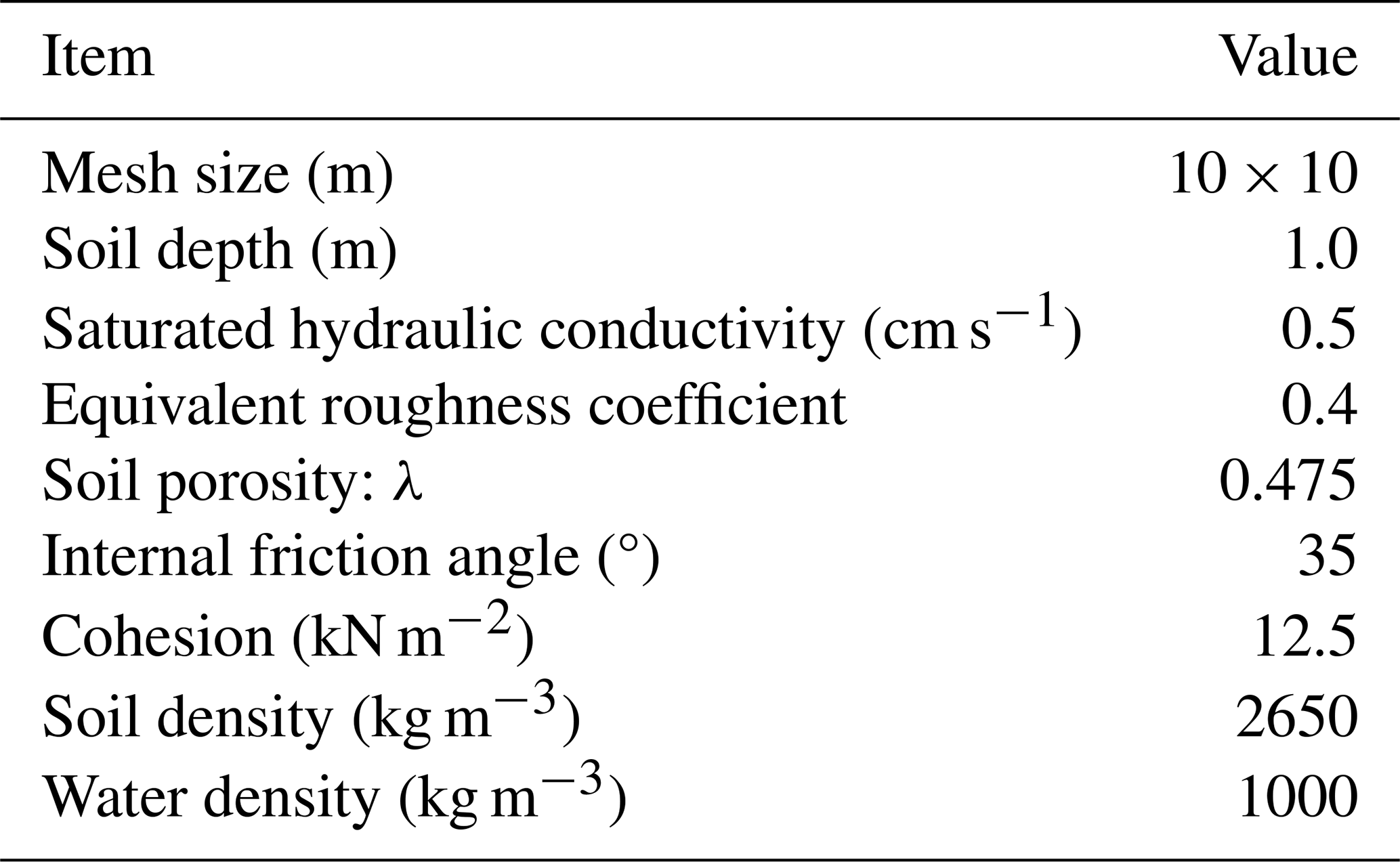
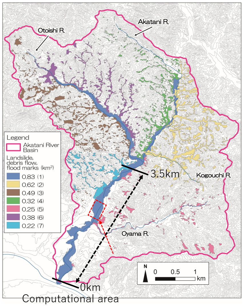
Figure 2The Akatani River basin with debris flows and flood marks identified from aerial photos (Nagumo and Egashira, 2019; was partially modified by the authors). The background image is provided by the Geographical Information Authority of Japan.
2.2 Evaluation of flood flow with sediment and driftwood
In order to create flood hazard maps for these hazards, we employ the depth averaged 2-D numerical simulations. The flow field is simulated using 2-D depth-integrated governing equations, which include mass and momentum conservation equations (e.g., Shimizu et al., 2019). The upstream boundary conditions for the 2-D computation are obtained by the methods in Sect. 2.1, in which we obtain a time series of sediment and driftwood discharged from the watershed. The 2-D forms of the Eqs. (2) and (3) are employed to evaluate the driftwood behaviour.
3.1 Computational conditions
The proposed method is applied to evaluate the flood disaster in the Akatani river, 2017, where a large amount of sediment and driftwood was produced in the mountainous area, as shown in Fig. 2. Parameters employed for the rainfall-runoff and landslide calculation is shown in Table 1. Initial sediment size distributions set in the channel network are given as shown in Fig. 3, referring to the sediment size distributions observed after the flood. The density of standing trees for the driftwood runoff simulation is set as 0.06 (m3 m−2).
The 2-D flood flow simulations with sediment and driftwood are conducted within the 3.5 km section as shown in Fig. 2. For upstream conditions related to flow discharge, sediment, and driftwood, we use the watershed computation results at the 3.5 km location. Calculations are performed for the two cases, flow only (Case 1) and with sediment and driftwood (Case 2) to compare the differences in results depending on the presence of sediment and driftwood.
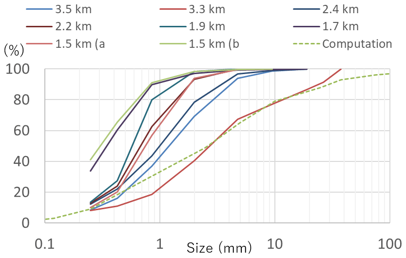
Figure 3Sediment size distribution in the riverbed surveyed after the disaster. The (km) in the legend is the distance from the Chikugo river confluence point, as shown in Fig. 2.
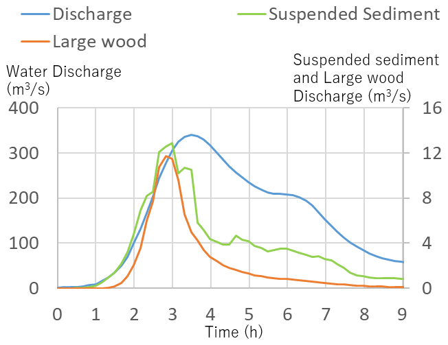
Figure 4Computational results of the watershed model for flood water, suspended sediment, and driftwood discharge at the 3.5 km point.
3.2 Results
Figure 4 shows the results of the watershed computation at 3.5 km point; the location corresponds to the upstream boundary of the 2-D flood flow computation. According to the figure, suspended sediment and driftwood discharge are concentrated around 3 h after the start of the event. This is due to the results that the occurrence of landslide and associated sediment transport are concentrated during this time period. This result is used as the upstream end boundary condition for the 2-D flood flow analysis, and the results in Fig. 4 indicate that a large amount of sediment and driftwood are discharged to the target section before the flood discharge reaches its peak flow.
Figure 5 compares the computational results for the inundation area between Case 1 and Case 2. There are seven bridges within the 3.5 km section, and the driftwood deposition in the computation exceeds 1 m in some of the bridges, thus the flow is obstructed, causing the flow to divert around the bridge. As a result, the inundation area in Case 2 is larger than that in Case 1, which is closer to the actual inundated area, shown as white dotted line.
Figure 6 compares the computation results at the peak flow with the water level marks to partially show the validity of this computation. In Case 2, the channel capacity has decreased due to sediment deposition on the river channel. Comparing the water levels in Case 1 and 2 with the water level mark, for example, around the 1.5 km location, where is the upstream of the bridge, Case 1 is about 1 m below the water level mark and Case 2 is about 50 cm above the water level mark. In Case 2, the bed shear stress in the river channel is reduced at upstream of the bridge due to the driftwood accumulation at the bridge, that causing significant sediment deposition here.
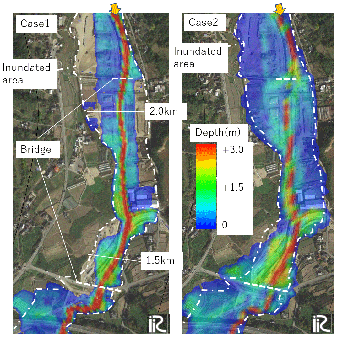
Figure 5Computational results of the water depth at peak discharge. The comparison is between Case 1 (flow only; left) and Case 2(with sediment and driftwood; right); The background image was taken from © Google Maps.
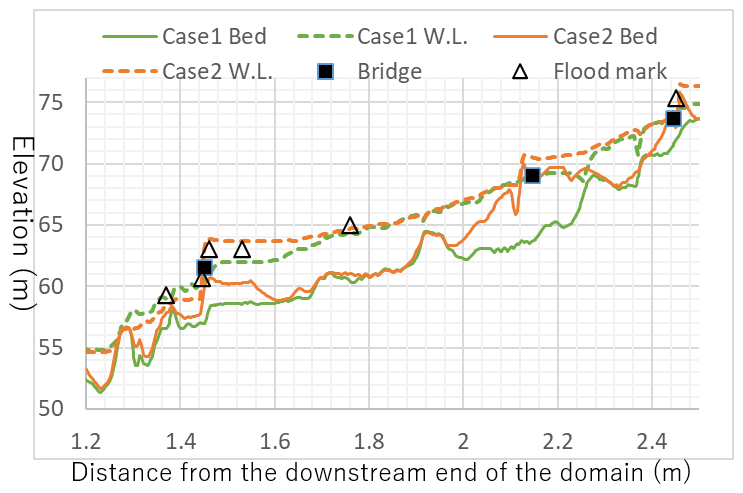
Figure 6Comparison of the results with the water level mark and river bed elevation in the longitudinal direction of the river channel during peak flow. Bridge location shows the elevation of the bridge.
Figure 7 compares the difference in sediment deposition during the flood event between the measured by an aerial laser survey (left figure) and the computational results in Case 2 (right figure). The trends in the two figures are generally consistent in terms that more than 2 m sediment deposition takes place in the river channel (red-coloured area) and that sediment is deposited several tens of centimeters thickness in the areas where inundation occurred.
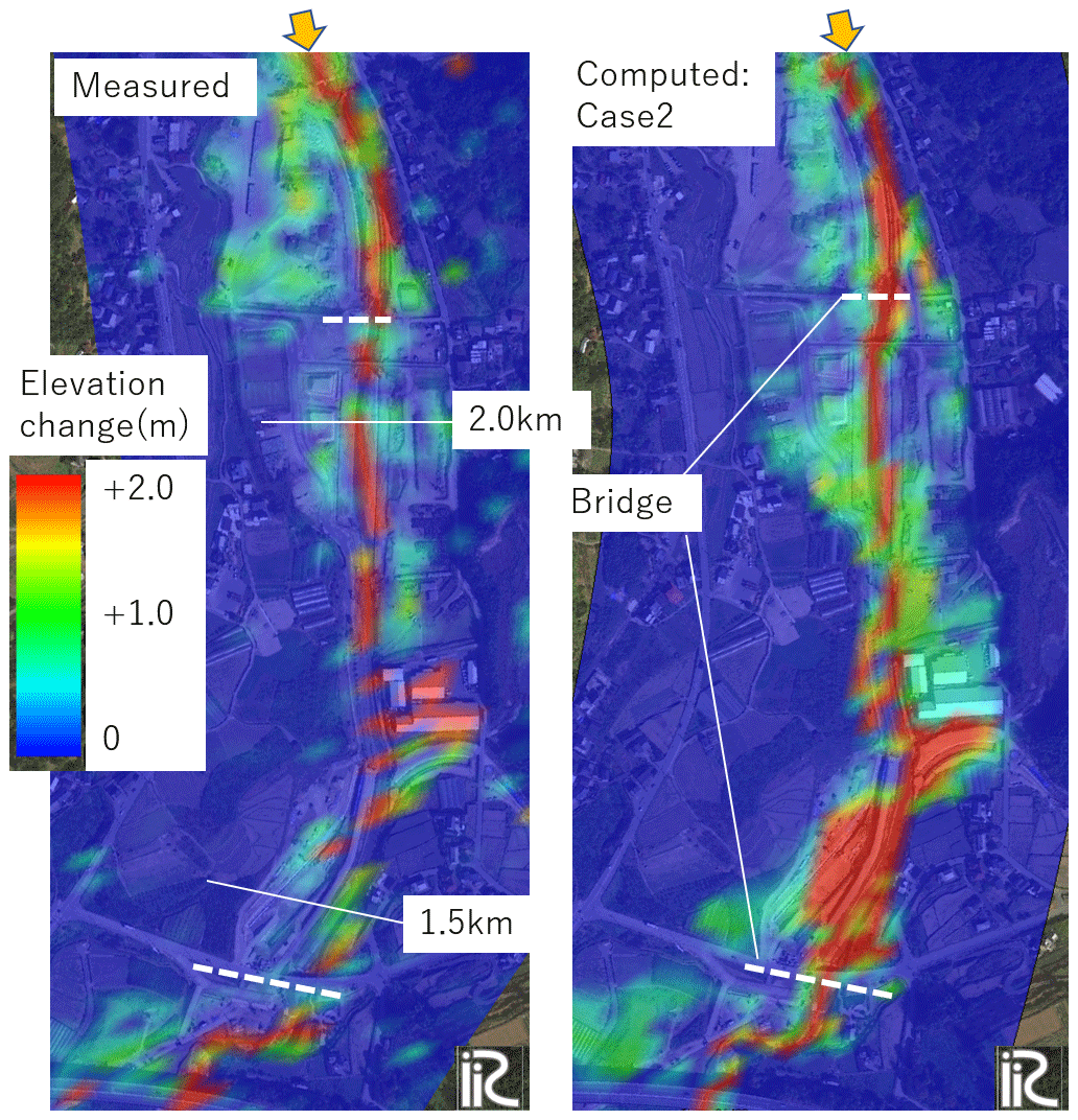
Figure 7Comparison of elevation changes before and after the flooding measured by aerial laser survey (left) and elevation change at the end of Case 2 computation (right). The background image was taken from © Google Maps.
In the Akatani River disaster, sediment conditions in the river channel changed drastically because of the large amount of fine sediment deposited in the channel supplied by landslide and debris flows in many places. According to Fig. 4, the supplied sediment is transported to the downstream, thus in the downstream river channels, this change seems to have occurred before the water discharge peak time. Figure 6 also shows that the river channel capacity is drastically reduced even before the flood flow peak comes, and the driftwood discharged from the watershed is deposited at the bridges, which significantly affect the water surface profile and flood flow around the bridges. To evaluate such a disaster, the physics-based method proposed in this study is effective.
Compared to existing methods for treating sediment and driftwood in the numerical simulation, this method allows us to perform physics-based integrated analysis of water, sediment, and driftwood runoff from the watershed. In particular, the unit channel concept in Fig. 1 and the convection equation in Eq. (2) allow the treatment of numerous amounts of sediment and driftwood transport. On the other hand, it should be mentioned that some challenges remain in creating hazard maps using such methods. For example, validation of the computed results is required where disasters have not yet occurred, thus validation should be conducted using the existing data for the present sediment transport or past disasters. Particularly, parameters that affect the results such as the soil cohesion, and sediment size distribution that we give as conditions should be carefully investigated in future.
In this research, we proposed methods to create flood hazard maps with active sediment and driftwood transport, using a watershed model and a 2-D flood flow model, where the driftwood transport is based on the convection and storage equations, and applied the methods to the Akatani river flood disaster in 2017 to discuss their applicability and challenges. As a result, the 2-D flood flow simulation that uses the results of watershed water, sediment, and driftwood runoff simulation reproduces the disaster in terms of inundation area, water depth, and sediment deposition. The methods proposed in this study are suitable for creating flood hazard maps in cases where the sediment conditions in the river channel change drastically, as in the case of the Akatani river disaster. However, further studies will be required for the use of practical hazard map creation in terms of the validation where disasters have not yet occurred, sediment size distribution, sediment sorting processes, river bank erosion, and so on.
The data are available from the corresponding author on reasonable request.
DH and SE conceptualized the study; DH performed the numerical simulations; DH wrote the manuscript draft; SE reviewed and edited the manuscript.
At least one of the (co-)authors is a guest member of the editorial board of Proceedings of IAHS for the special issue “ICFM9 – River Basin Disaster Resilience and Sustainability by All”. The peer-review process was guided by an independent editor, and the authors also have no other competing interests to declare.
Publisher's note: Copernicus Publications remains neutral with regard to jurisdictional claims made in the text, published maps, institutional affiliations, or any other geographical representation in this paper. While Copernicus Publications makes every effort to include appropriate place names, the final responsibility lies with the authors.
This article is part of the special issue “ICFM9 – River Basin Disaster Resilience and Sustainability by All”. It is a result of The 9th International Conference on Flood Management, Tsukuba, Japan, 18–22 February 2023.
The authors would like to thank Naoko Nagumo, Yousuke Nakamura, and Yusuke Yamazaki for their contribution to the field survey and data preparation for this study.
This research has been supported by the Japan Society for the Promotion of Science (grant no. 22K14334).
This paper was edited by Kensuke Naito and reviewed by Dimitrios Fytanidis and one anonymous referee.
Comiti, F., Mao, L., Preciso, E., Picco, L., Marchi, L., and Borga, M.: Large wood and flash floods: evidence from the 2007 event in the Davča basin (Slovenia), WIT Transactions on Engineering Sciences, 60, 173–182, 2008.
Egashira, S. and Matsuki, T.: A method of predicting sediment runoff caused by erosion of stream channel bed, Annual Journal of Hydraulics Engineering, Japan Society of Civil Engineers, 44, 735–740, 2000 (In Japanese).
Harada, D. and Egashira, S.: Flood flow characteristics with fine sediment supply and drift woods – analysis on the akatani river flood hazards in july, 2017, Annual Journal of Hydraulic Engineering, Japan Society of Civil Engineers, 74, I_937–I_942, 2018 (in Japanese).
Huang, R., Ni, Y., and Cao, Z.: Coupled modeling of rainfall-induced floods and sediment transport at the catchment scale, Int. J. Sed. Res., 37, 715–728, 2022.
Liu, H., Du, J., and Yi, Y.: Reconceptualising flood risk assessment by incorporating sediment supply, CATENA, 217, 106503, https://doi.org/10.1016/j.catena.2022.106503, 2022.
Lucía, A., Schwientek, M., Eberle, J., and Zarfl, C.: Planform changes and large wood dynamics in two torrents during a severe flash flood in Braunsbach, Germany 2016, Sci. Total Environ., 640, 315–326, https://doi.org/10.1016/j.scitotenv.2018.05.186, 2018.
Nagumo, N. and Egashira, S.: Flood Hazard Analysis and Locations of Damaged Houses Based on Land Classification in the Akatani River Basin Following Torrential Rainfall in Northern Kyushu, 2017, Journal of Geography (Chigaku Zasshi), 128, 835–854, 2019 (in Japanese).
Sayama, T., Ozawa, G., Kawakami, T., Nabesaka, S., and Fukami, K.: Rainfall–runoff–inundation analysis of the 2010 Pakistan flood in the Kabul River basin, Hydrol. Sci. J., 57, 298–312, 2012.
Shimizu, Y., Nelson, J., Arnez Ferrel, K., Asahi, K., Giri, S., Inoue, T., Iwasaki, T., Jang, C.L., Kang, T., Kimura, I., and Kyuka, T.: Advances in Computational Morphodynamics Using the International River Interface Cooperative (iRIC) Software, Earth Surf. Process. Landf., 45, 11–37, https://doi.org/10.1002/esp.4653, 2019.
Yamazaki, Y. and Egashira, S.: Run out processes of sediment and woody debris resulting from landslides and debris flow, Association of Environmental and Engineering Geologists, special publication 28, 2019.