Streamflow simulation using the event-based SCS-MS/LR model in the Hitiaa catchment, French Polynesia

The volcanic tropical Island of Tahiti is prone to heavy rainfalls and flash floods which regularly generate severe damages. Hydrological response on the island is highly variable from one catchment to the other, in terms of runoff production as well as peak flow amplitude. Infrastructures designers there require an operational method able to calculate the design flood metrics on any Tahitian catchment, taking into account the variability of their response. This study applies a parsimonious distributed event-based conceptual model to the observed rainfall-runoff events of 9 small catchments (<6 km²). A modified version of the Mishra and Singh Soil Conservation Service (SCS-MS) runoff model, associated with the Lag-and-Route (LR) model was applied to series of 9 to 176 rainfall-runoff events for each catchment that occurred between 2004 and 2021. Two dominant parameters are to be considered for the SCS-MS model: the size of the soil reservoir (Si) and the initial water content (M) in this soil reservoir. SCS-MS was found to perform better than SCS-CN and to fit better the asymptotic behaviour of the rainfall-runoff relationship. Si could be fixed to 2500 mm for all catchments except Nymphea where Si had to be lowered to 80 mm, because of the high density of urbanization over this catchment. M parameter was set variable from one event to the other as the initial condition of the model. The Nash criterion was calculated for each event and their median value ranged from 0.39 to 0.79 across the catchments, proving the flexibility of the model. A clear relationship could be fitted between the median M and Antecedent Precipitation Index (API), both calculated for each catchment. Further testing of this model on similar tropical volcanic context should be undertaken to verify its flexibility and to consolidate the calibration of its parameters.

1 Introduction

Flash floods have been recognized as the main natural risk in the Island of Tahiti, where high urbanization rate increases the vulnerability of people, homes and infrastructures (Lamaury et al., 2021). There is a strong need for a flood predetermination method to assist engineers in the design of hydraulic infrastructure.

Flash floods result from the combined effects of extreme rainfall events and the steep morphology of the catchments (Wotling, 1999). However, their relative influences on the hydrological response and the variability of these influences across the island have not yet been captured by a rainfall-runoff model.

Wotling (1999) and Pheulpin (2016) verified the ability of event-based distributed conceptual models to reproduce the hydrological response of three western and one southern catchment. The low number of studied catchments didn't allow them to explain the spatial variability of hydrological response, nor to relate the model parameters to measurable characteristics of the catchment such as geomorphology, soil moisture, altitude or exposure to trade winds.

The main objective of this study is to select and apply a rainfall-runoff model that is both robust to the hydrological variability in Tahiti and ready to be regionalized. The chosen model should be parsimonious to facilitate its transfer to ungauged catchments, and its parameters are to be related to physical features of the catchments.

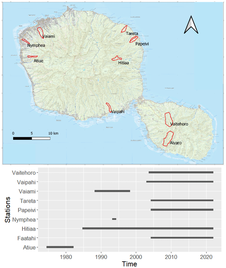
Figure 1 Location of the gauged catchments chosen to calibrate the rainfall-runoff model, and record periods of the associated discharge stations. IGN map available at (https://www.data.gouv.fr/fr/datasets/r/3aad9e99-50f8-4bb1-8b27-2cf3b19301af, last access: 20 November 2021).

2 Study site and data

2.1 The island of Tahiti

Tahiti is a volcanic island belonging to the Society Archipelago in the middle of the Pacific Ocean. Tahiti is the biggest – area of 1042 km² –, the highest – Mount Orohena culminates at 2241 m – and the most populous – 192 760 inhabitants in 2017 – island of French Polynesia. The Island is subject to a southern tropical climate, controlled by northeasterly trade winds and the South Pacific Convergence Zone. Rainfall pattern is very heterogeneous within the island, and it is also the case for extreme events. Wotling (1999) and Pheulpin (2016) modelled extreme rainfall events from topography and exposure to trade winds.

2.2 Studied catchments

Over the 33 catchments that are or have been gauged in Tahiti, nine catchments were chosen to test and calibrate the rainfall-runoff model. Record periods are indicated in Fig. 1.

They were selected for the quality of the data and because they are small-sized catchments, with area lower than 6 km². Thus their area is considered small enough to neglect the variability of physio-climatic variables within them, so that each of them can be representative of a specific environment, at least in terms of altitude and rainfall input.

Locations of the catchments are selected in order to capture the spatial variability of rainfall exposure within the island. Both leeward and windward sides of the main island – Tahiti Nui – are considered, as well as the peninsula – Tahiti Iti.

Figure 2 Spatial variability of hydrologic behaviours: Cumulative rainfall and runoff of events extracted from observation data in the studied catchments. Number of events of each series is indicated next to the name of the catchment.

Each catchment is instrumented with one or two rain gauges and the rainfall is interpolated by the Thiessen method. For each catchment, series of events are extracted at a 5min timestep from the rainfall and flow records. An event is extracted if it occurs after a duration of at least 3 h with rainfall intensity below 0.3 mm in 5 min. Cumulative rainfall and runoff must exceed thresholds that are adjusted from one catchment to the other so that the number of collected events is enough. The direct runoff volume for each event is then calculated by subtracting the base flow from the total instantaneous flow. Resulting runoff coefficients highlight the variability of the hydrological response among the selected catchments (Fig. 2).

3 Rainfall runoff model

The Mishra et al. (2003) Soil Conservation Service (SCS-MS) runoff model was modified and associated with the Lag-and-Route (LR) model to simulate the complete flood hydrographs. Note the model operates for each cell of a regular grid mesh. Each cell produces an elementary hydrograph, and the addition of all the elementary hydrographs leads to the complete flood hydrograph.

3.1 SCS-CN and SCS-MS model

Original SCS is based on the following equations:

$$\begin{array}{}\text{(1)}& {\displaystyle }P=\mathrm{Ia}+F+Q\text{(2)}& {\displaystyle \frac{Q}{P-\mathrm{Ia}}}={\displaystyle \frac{F}{S}}\text{(3)}& {\displaystyle }\mathrm{Ia}=\mathit{\lambda }S\end{array}$$

with P standing for total precipitation, “Ia” for initial abstraction, F for cumulative infiltration, Q for direct runoff, S for potential maximum retention.

Combined together, Eqs. (1), (2) and (3) lead to:

$$\begin{array}{}\text{(4)}& Q={\displaystyle \frac{{\left(P-\mathrm{Ia}\right)}^{\mathrm{2}}}{P-\mathrm{Ia}+S}}\end{array}$$

Mishra and Singh (2003), introduced the concept of equality between the runoff coefficient C and the degree of saturation Sr. Sr being expressed as:

$$\begin{array}{}\text{(5)}& Sr={\displaystyle \frac{F}{S+M}}\end{array}$$

with M the initial soil moisture, and C as:

$$\begin{array}{}\text{(6)}& C={\displaystyle \frac{Q}{P}}\end{array}$$

Equation (2) of the SCS becomes:

$$\begin{array}{}\text{(7)}& {\displaystyle \frac{Q}{P-\mathrm{Ia}}}={\displaystyle \frac{F+M}{S+M}}\end{array}$$

The total soil reservoir capacity Si was introduced as:

$$\begin{array}{}\text{(8)}& \mathrm{Si}=S+M\end{array}$$

Equation (4) of the SCS is rewritten for the SCS-MS as follows:

$$\begin{array}{}\text{(9)}& Q={\displaystyle \frac{\left(P-\mathrm{Ia}\right)(P-\mathrm{Ia}+M)}{P-\mathrm{Ia}+S+M}}\end{array}$$

Figure 3 Conceptual diagram of the modified SCS-MS production function.

Equation (4) was then differentiated as a function of time to calculate the direct runoff at each timestep. To adapt them to the dynamic flow calculation, the SCS-MS equations have been modified in the same way as in the work of Coustau et al. (2012):

• To take into account the potential decrease of the runoff coefficient between floods, the cumulative rainfall P (t) is considered as the level of a reservoir of infinite capacity to which an emptying is applied:

  $$\begin{array}{}\text{(10)}& {\displaystyle \frac{\mathrm{d}P\left(\mathrm{t}\right)}{\mathrm{d}t}}=P_{\mathrm{b}}\left(t\right)-\mathrm{d}s.P\left(\mathrm{t}\right)\end{array}$$

  where ds [T⁻¹] is the linear decay coefficient and P_b (t) is the input rainfall intensity.

• Soil drainage is represented by the application of a drain modulated by the same coefficient ds:

  $$\begin{array}{}\text{(11)}& {\displaystyle \frac{dH\left(\mathrm{t}\right)}{\mathrm{d}t}}=P_{\mathrm{b}}\left(\mathrm{t}\right)-R_{\mathrm{dir}}\left(\mathrm{t}\right)-\mathrm{d}s.H\left(\mathrm{t}\right)\end{array}$$

  where R_dir (t) [L T⁻¹] is the direct runoff intensity.

• Delayed flow R_del is introduced by recovering a fraction ω of the soil discharge at the outlet:

  $$\begin{array}{}\text{(12)}& R_{del}\left(\mathrm{t}\right)=\mathit{\omega }.\mathrm{d}s.H\left(\mathrm{t}\right)\end{array}$$

  where ω is a dimensionless exfiltration coefficient.

5 parameters are associated to SCS-MS: Si, Ia, M, ds and ω.

3.2 Lag and Route model

The Lag-and-Route model (Maidment, 1993) routes the runoff production of each cell m to the outlet of the catchment.

Figure 4 Lag-and-Route transfer function (modified from Maidment, 1993).

According to the production function, each cell produces an elementary hydrograph at each time t,equation can be written as:

$$\begin{array}{}\text{(13)}& \begin{array}{l}\left\{\begin{array}{l}{Q}_{\mathrm{m}}\left(\mathrm{t}\right)=\mathrm{0}\mathrm{if}t<t_{\mathrm{o}}+T_{\mathrm{m}}\\ Q_{\mathrm{m}}\left(\mathrm{t}\right)=\frac{R\left(t_{\mathrm{o}}\right)}{K_{\mathrm{m}}}\cdot \exp \left(-\frac{\left(t-(t_{\mathrm{o}}+T_{\mathrm{m}})\right)}{K_{\mathrm{m}}}\right).A\end{array}\mathrm{otherwise}\right.\end{array}\end{array}$$

where R(t_o) is the runoff produced by the m cell at time t_o, T_m is the propagation time and K_m is the diffusion time. They are linked by the K₀ [–] constant as follows:

$$\begin{array}{}\text{(14)}& K_{\mathrm{m}}=K_{\mathrm{0}}\cdot T_{\mathrm{m}}\end{array}$$

T_m is the travel time from the m cell to the catchment outlet. It can be expressed by:

$$\begin{array}{}\text{(15)}& T_{\mathrm{m}}=\sum _{k=\mathrm{1}}^n{\displaystyle \frac{l}{V_{\mathrm{0}}}}\end{array}$$

where n is the number of cells of length l between the cell m and the outlet and V₀ is linked to the velocity of water transfer. V₀ and K₀ are the input parameters for the transfer function.

4 Model calibration

SCS-MS/LR was calibrated on each catchment from the series of observed rainfall-runoff events. 5 parameters must be calibrated for the production function (Si, Ia, M, ω and ds) and 2 parameters for the transfer function (V₀ and K₀). K₀ was arbitrarily fixed to 0.7 for all events and all catchments because highly related to V₀ (Coustau et al., 2012; Nguyen and Bouvier, 2019). Ia was fixed for all events and all catchments from graphical fit of the theoretical balance sheet equation (Eq. 9) on observations of event cumulative rainfall and runoff (Fig. 2). Si, ds and ω were first calibrated by trial and error and sensibility analysis over each series of events paying attention to the median value of the NSE criterion (Nash and Sutcliffe Efficiency, Nash and Sutcliffe, 1970). Explored ranges of values are from 0.01 to 0.6 for ω, from 0.5 to 2 m s⁻¹ for ds and from 10 to 3000 mm for Si, based on previous applications of the SCS model (Coustau et al., 2012; Nguyen and Bouvier, 2019). Then these three parameters were uniformed for all catchments when possible in order to reduce the risk of equifinality.

Parameter M stands for the initial condition of the model, and should vary from one event to the other. According to its physical meaning, V₀ should also be set variable from one event to the other. These two state parameters should be related to initial conditions like the level of soil humidity at the beginning of each event. For each catchment, such initialization relationships were built between optimized values of M and V₀ on one hand, and measured baseflow Q₀ at the beginning of each event on the other hand. Q₀ is used here as a proxy for Antecedent Moisture Conditions.

Parameters M and V₀ were simultaneously optimized for each event, using the SIMPLEX method (Nelder and Mead, 1965) and NSE as efficiency criterion. SIMPLEX explores the parameter space and converges to a pair of final parameters (M, V₀) either after 300 iterations or when the difference in NSE between two successive iterations is less than 10⁻⁹.

5 Results

5.1 Improvement of the SCS-MS model compared to the SCS

Before calibrating the SCS-MS/LR model in dynamics, its balance equation (Eq. 9) is adjusted for each catchment on the observed event rainfall and runoff totals. The objective is to calibrate Ia parameter and to verify that the SCS-MS can adapt to the diversity of hydrological behaviours that can be observed in Tahiti. Compared to the SCS equation (Eq. 4), SCS-MS fits better the whole range of observed rainfall-runoff events, especially for catchments with the lowest observed runoff coefficient like Vaipahi. For these catchments, SCS has a tendency to under-estimate the low flow events when SCS-MS crosses the scatterplot at its centre (Fig. 5).

Figure 5 Comparative fits of the SCS and SCS-MS models on event cumulative rainfall and runoff observed in the Vaipahii catchment.

With Ia parameter greater than 0, balance equations of both models proved to be inadequate to fit observations, especially for catchments with observed runoff coefficients below 0.4. Ia parameter was then set to 0 for both models.

5.2 Parameter calibration and model efficiency

To measure the efficiency of SCS-MS/LR on each catchment, NSE was calculated for each event, and then the median of the NSE was calculated over each series of events.

Figure 6 Distribution of Nash coefficients for each catchment, with M and Vo being optimized (a) and fixed to median values of optimized sets (b).

SCS-MS/LR model showed little sensitivity to the parameters ds, ω and Si. It was therefore possible to find uniformed values of these parameters over the range of catchments. ds and ω were set to 1 d⁻¹ and 0.2 respectively, and Si could be set to 2500 mm for all basins except Nymphea. For Nymphea, the optimal value of Si is 80 mm, and setting the NSE to 2500 degrades the median of NSE criterion from 0.77 to 0.08. For the other catchments, setting Si at 2500 mm leads to negligible degradation of median NSE, which remains above 0.73 (Fig. 6).

Initialization relationships between Q₀ and optimized values of V₀ and M parameters were found not robust enough to be retained: R² coefficients of the adjusted relationships were found lower than 0.1 for 6 catchments out of 9 for M, and lower than 0.1 for all catchments for V₀. The model is therefore unable to reproduce the temporal variability of the hydrological response, but it remains relevant for characterize the median hydrological behavior of each catchment. For each catchment, M and Vo were therefore set to the medians of the optimised sets. Median M varies between 8 and 1710 mm depending on the catchment, and Vo varies between 0.9 and 1.6 m s⁻¹. These two parameters are not correlated, which is reassuring with regard to the risk of equifinality.

Median NSE values ranged from 0.73 to 0.87 across the catchments when M and V₀ optimized and from 0.39 to 0.79 with M and V₀ fixed to the median of optimizes values (Fig. 6).

Setting Vo and M to a single value for each basin lowers the NSE criteria because the model no longer takes into account the temporal variability of the hydrological response. The poor performance of the relationships between these two parameters and the AMC proxy can be explained by the existence of spatial uncertainties in rainfall that interfere with the optimisation of M and Vo. Rainfall patterns in Tahiti are highly variable in space (Benoit et al., 2022) and a high level of uncertainties is associated with values of spatial rainfall averages. These uncertainties are reflected in the hydrological model on the optimization of the initial condition until blurring the relationship between the initial condition and a proxy for AMC (Tanguy et al., 2023).

5.3 Towards the regionalization of the model parameters

After calibrating M and Vo separately for each catchment, their spatial variability, attempts were made to explain their spatial variability. The median values of M were linked to a proxy of AMC in order to explain its spatial variability across catchments.

Relationship between median M and median Q₀ was not relevant, but a clear relationship was identified between the median M and the mean Antecedent Precipitation Index (API) calculated separately for each catchment (Fig. 7). API was formulated by Fedora and Beschta (1989) as follows:

$$\begin{array}{}\text{(16)}& {\mathrm{API}}_{\mathrm{t}}=\left({\mathrm{API}}_{\mathrm{t}-\mathrm{\Delta }t}\mathrm{K}\right)+P_{\mathrm{\Delta }t}\end{array}$$

K is a recession constant that we fixed to 0.85. We calculated API at a daily time step for the rainfall time series of each catchment, before extracting the daily API corresponding to the day before the beginning of each rainfall event.

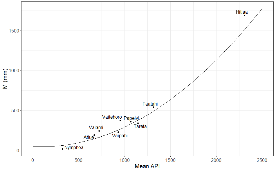
Figure 7 Adjustment of a relationship between the median M parameter calculated for the series of event of each catchment, and the mean API (Antecedent Precipitation Index), also calculated for each event series.

A hypothesis to explain the low Si value in the Nymphea catchment lies in the difference of land use. The land use type of each catchment was estimated from satellite images of the island (Google maps). All catchments are mainly natural with peri urban areas smaller than 20 % of the total catchment surface, except Nymphea which is the only catchment to be entirely urbanized. Reducing the size Si of the soil reservoir for urban basins is coherent since artificial surfaces are mostly impermeable. Surface runoff is favoured compared to natural basins where an increased production capacity allows more infiltration, storage and subsurface runoff.

6 Conclusions

The modified version of SCS-MS/LR was calibrated and tested on series of observed rainfall-runoff events from 9 Tahitian catchments. V₀ and M could not be initialized from AMC proxy, and had to be fixed for each catchment. The model no longer restitute the temporal variability of rainfall-runoff response, but is still relevant to provide the average behavior of each catchment. Evaluated by the median values of NSE calculated for each catchment, the model efficiency is affected by the approximation made on V₀ and M but remains above 0.39. This model fulfills the flexibility required to restitute the hydrological spatial variability in Tahiti and its small number of parameters makes it a good candidate for regionalization.

About the regionalization of the model parameters, Si can be set according to the land use type. The median M is significantly related to the average API, which is a proxy for the average moisture state of each catchment. This study presents soil moisture as a key variable to regionalize rainfall-runoff models. However, the regionalization is not completed because V₀ spatial variations still remain unexplained, and because the model has not been validated.

This model and the relationship found between M and mean API are promising for event rainfall-runoff modelling in tropical volcanic context. However, it could be applied to other catchments in similar context in order to consolidate the calibration of its parameters and to clarify the regionalization relationships. The impact of land use type on the Si parameter could especially be specified.