Tracing and hydraulic modelling to assess the hydraulic performance of a constructed wetland

Constructed wetlands are widely used to protect sensitive water resources from non-point source pollution from agriculture. Their potential to remove nitrate and pesticides increases with the water residence time and a uniform distribution of the inflow over the wetland area. Over the hydrological season, inflow variations greatly modify the theoretical residence time. The knowledge of the corresponding variations of the hydraulic performance constitutes a gap for the better management of treatment wetlands, especially for wetland with heterogeneous vegetation implementation. The aim of this work is to investigate how the hydraulic performance changes with the flow rate in a partly vegetated wetland. The study site, a 0.5 ha wetland, is located in an area of intensive cereal crop production in Northern France. The three-dimensional hydrodynamic model Delft3D-Flow was used to simulate flow through vegetation, forced by observed meteorological conditions. It was calibrated on continuous outflow concentration measurements and unmanned aerial vehicle (UAV) images during a 13 d tracing experiment with rhodamine WT. The simulated hydraulic performance indicators matched satisfactorily with observed values thanks to the detailed description of the vegetation. Simulations for the locally usual flow range and for a fixed water depth showed a limited increase of the hydraulic performance with the flow rate. This shows that conducting a tracing at low flow is sufficient to assess the average hydraulic performance of a wetland.

1 Introduction

A promising measure against non-point source pollution from agriculture, complementary to the reduction of fertilizers and pesticides applications, is the implementation of constructed wetlands intercepting polluted surface water (Tournebize et al., 2017). They are widely used to protect sensitive water resources (e.g. aquifers, lakes or rivers), especially when grass strips are bypassed by a subsurface drainage network. Constructed wetlands, intermittently fed during autumn and spring in a temperate climate, are composed of three interacting compartments: sediment layer, vegetation and water column. Pollutant mitigation increases with the time spent by water in contact with the sediment and with vegetation. The pollutant removal potential is mainly driven by the inflow rate and by its uniform distribution over the wetland area. When sparse or in patches, vegetation makes the flow path complex and can cause bypasses and dead zones in the wetland, and consequently affects its hydraulic performance. The scientific challenge is to link the yearly patterns of discharge, hydraulic performance and removal rate, in order to provide guidelines for the design of constructed wetlands.

Most literature about waste stabilization ponds and other constructed wetlands is based on laboratory experiments and two-dimensional hydraulic simulations at constant flow rate and homogeneous mass density (for a review: Ho et al., 2017). For surface free wetland, vertical flow stratification and mixing due to bathymetry, inflows, weather conditions and vegetation are often neglected, while they can have considerable consequences: Sweeney et al. (2003)'s three dimensional simulations showed that wind could change the residence time distribution from quasi plug flow into quasi fully mixed flow in a large waste stabilization pond, with high effects on the treatment efficiency; Adamsson et al. (2005) attributed the unexpectedly high residence time of a tracer at low flow in a laboratory tank to the deep storage of the cool inflow. Bulat et al. (2019) applied a three-dimensional model for the flow within rigid emergent and submerged vegetation to a large fluvial lake and showed the improvement of stratified flow description compared to the usual representation with a Manning-Strickler bottom roughness.

Holland et al. (2004) found experimentally that the flow rate had little impact on the hydraulic performance of a non-vegetated constructed wetland. The aim of this work is to investigate whether this is still true in a vegetated shallow wetland, using a three-dimensional model.

2 Material and methods

2.1 Study site and instrumentation

The study site is the wetland (0.53 ha) constructed in 2010 in Rampillon, 60 km South-East of Paris, France (Fig. 1, Tournebize et al., 2012). This wetland is a buffer zone between a 355 ha drained agricultural catchment and a direct recharge zone into a karstic aquifer through sinkholes (Mander et al., 2021). At full capacity, the depth of the compartments ranges from 0.5 (for the main compartment) to 1.2 and 1.5 m (for the inlet and outlet compartments). While the inlet is located above the water surface, the outlet collects water at mid-depth to avoid the clogging by floating vegetation. Baffles are intended to avoid short-circuits between inlet and outlet. Since the initial planting (juncus, carex and typha), the vegetation has developed naturally and, partially degraded by animals, became sparse and highly heterogeneous. At time experiment, vegetation cover was estimated to 39 % of total wetland area.

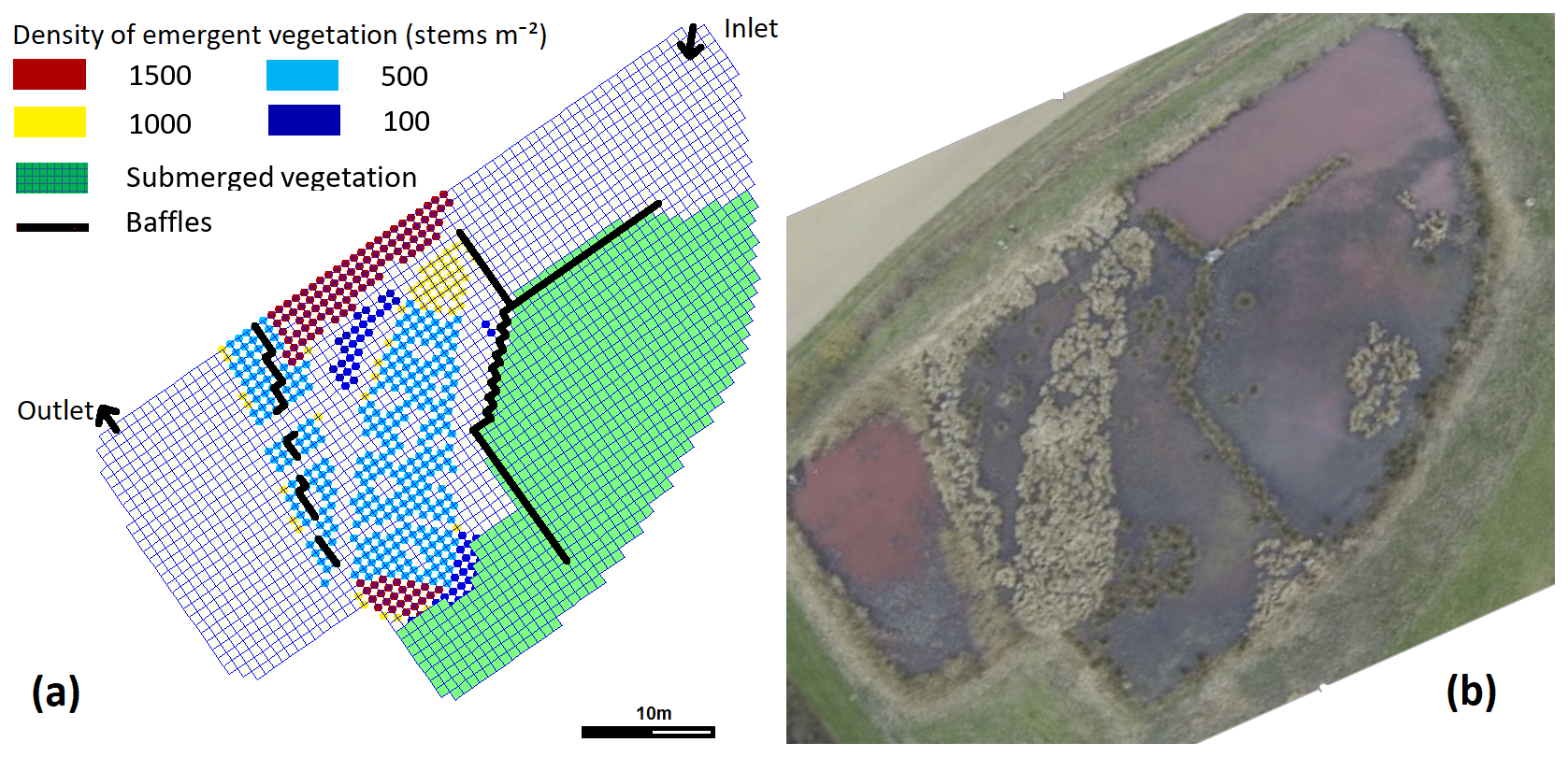
Figure 1 (a) Mesh and representation of the baffles and of vegetation inside the wetland (The pink arrow represents the longitudinal cross-section used in Fig. 4), (b) UAV image of the wetland, 48 h after the tracer injection.

2.2 Tracing experiments

204 g of the conservative tracer Rhodamine WT were injected on 22 March 2016, between 07:10 and 10:15 local time. The outflow rate, recorded every 15 min during the tracing (Sigma 950 AV flow meter), varied from 3 to 10 L s⁻¹ over the first nine days (average 6.6 L s⁻¹), then peaked at 70 L s⁻¹ after a rain event (Fig. 2). The theoretical residence time computed on these first nine days from the mean volume and flow rate was around 3.5 d. The tracer concentration was continuously monitored for 13 d with a fluorimeter (GGUN FL30), with a recovery rate of 94 %.

UAV images (11 images during the first day, and one each of the following 2 d) captured the flow paths within the wetland. The average water depth during the first nine days was only 0.1 m in the main compartment, so that the velocity averaged across the main flow direction was in the range of 10⁻³ m s⁻¹ (Reynolds number around 100, laminar flow). It increased to around 10⁻² m s⁻¹ in preferential flow areas (turbulent flow).

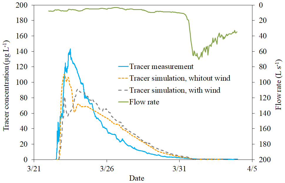
Figure 2 Residence time distribution measured during the winter tracing (2016) and simulated by the model and flow rate entering the wetland.

2.3 Model configuration

The three-dimensional hydrodynamic model Delft3D-Flow (version 4.01.01.rc.03, Deltares, 2014) was used to simulate flow within the constructed wetland. This model has proven ability to simulate the hydrodynamics, the stratification and the mixing of shallow lakes (Soulignac et al., 2017). It describes the flow through emergent and submerged vegetation (Bulat et al., 2019).

The model assumes a hydrostatic pressure distribution and solves the Reynolds-averaged Navier-Stokes equations for an incompressible fluid with the Boussinesq approximation and a turbulence-closure model, here the k-ε model. The mesh was composed of about 2500 1.5 m ×1.5 m cells and 10 horizontal layers. Their thickness increases exponentially from top to bottom (6 % to 16.5 % of the total height) for the description of flow stratification.

In this model configuration, viscosity and diffusion are isotropic; they are the sums of a molecular term, kinematic viscosity and molecular diffusivity, and of the k-ε eddy viscosity and diffusivity respectively. Contrary to other studies with more turbulent flow (e.g., Soulignac et al., 2017), turbulence within the large cells was neglected (background horizontal eddy viscosity and diffusivity). Rhodamine WT was simulated as a passive tracer.

Due to unreliable measurements of the inflow rate, it was computed from the outflow rate and water depth measurements. Both inflow and outflow rates were forced in single cells at the inlet and outlet to ensure numerical stability; the temperature measured in the inlet pipe was used as input in the model.

Surface energy balance is represented by Delft3D “Ocean model”. It was forced by daily SAFRAN reanalyses (air humidity and temperature, solar radiation) (Raimonet et al., 2017) and by hourly wind speed and direction from the nearest weather station of Melun, 32 km away.

Delft3D rigid vegetation module represents flow in vegetation (Bulat et al., 2019): the drag caused by vegetation is proportional to the stem density and diameter and creates a rather uniform current speed profile along the stems as opposed to the usual logarithmic profile. We placed patches of submerged (20 cm high) and emergent vegetation according to UAV images and in situ observation, we fixed their stem diameter to 5 mm and kept their stem densities as calibration parameters (Fig. 1a).

The roughness of the bottom of the wetland was represented by a Manning coefficient computed after Arcement and Schneider (1989), with a value of 0.3 s m${}^{-\mathrm{1}/\mathrm{3}}$ under submerged vegetation, else of 0.01 s m${}^{-\mathrm{1}/\mathrm{3}}$ (settled fine sediment). The free slip condition was adopted for banks and baffles, the latter represented as thin dams. Due to animals (nutria, Myocastor coypus) digging breaches in the baffles, short-circuits are clearly visible on UAV images (not shown). These breaches were represented in the model (Fig. 1a).

Water was initially set at rest and at the daily air temperature (7.5 °C); the warming up period was 8 h. The time step was 6 s to fulfill the Courant-Friedrichs-Lewy condition.

2.4 Hydraulic performance indicators

This subsection presents the extraction of hydraulic performance indicators from the residence time distribution C(t), where C is the tracer concentration and t the time elapsed since the beginning of injection. Dimensionless flow-weighted time φ and concentration C^′ make it possible to compute the theoretical and the effective mean residence time in varying outflow rate Q and retention volume V (Holland et al., 2004):

$$\begin{array}{}\text{(1)}& \mathit{\phi }=\underset{\mathrm{0}}{\overset{t}{\int }}{\displaystyle \frac{Q\left(t^{\prime }\right)}{V\left(t^{\prime }\right)}}\mathrm{d}{t}^{\prime }\end{array}$$

$$\begin{array}{}\text{(2)}& C^{\prime }\left(\mathit{\phi }\right)={\displaystyle \frac{C\left(\mathit{\phi }\right)V\left(\mathit{\phi }\right)}{M_{\mathrm{out}}}}\end{array}$$

where M_out is the total mass recovered over the tracer monitoring time T.

The first indicator is the dimensionless mean residence time φ_m, also called effective volume ratio:

$$\begin{array}{}\text{(3)}& {\mathit{\phi }}_{\mathrm{m}}=\underset{\mathrm{0}}{\overset{T}{\int }}\mathit{\phi }{C}^{\prime }\left(\mathit{\phi }\right)\mathrm{d}\mathit{\phi }\end{array}$$

The second one, a short-circuit index, is the dimensionless time of the 1st decile of the tracer mass, φ_10 %. The third one, a mixing indicator, is the dimensionless delay between the 1st and last deciles of the tracer mass, φ_90 %−φ_10 %. Teixeira and do Nascimento Siqueira (2008) experimentally showed that these were more reliable than most other indicators.

2.5 Model calibration and wetland hydraulic performance

During the calibration, only the vegetation stem density was triggered, in steps of 100 stems m⁻². In a first phase, we reproduced qualitatively the flow pattern visible in the UAV images and the overall shape of the residence time distribution, especially the timing of the peaks (Fig. 2). Then, a second phase consisted in fitting the hydraulic indicators, with and without wind input. The water level evolution was checked at the end of modelling.

The calibrated model was then used to test whether hydraulic performance changes with the flow rate within its annual range in the study area, excluding high flows. Tracing simulations were run for different constant flow rates from 10 to 60 L s⁻¹, with the average water depth and the weather conditions observed during the tracing, but without wind.

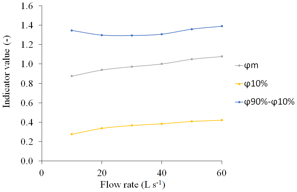
Figure 3 Evolution of simulated indicators (mean residence time, short-circuit and mixing indicators) with the flow rate.

3 Results

3.1 Performance of the calibrated model

Model calibration made it possible to fit the simulated residence time distribution with the observations (Fig. 2). The recovery rate of the tracer is satisfactory (97 % in the simulations). While results were poor with a Manning-Strickler description of vegetation (data not shown), the simulated residence time distribution and hydraulic indicators matched observations after calibrating the vegetation density. Suppressing the wind input improved the shape of the residence time distribution (Fig. 2). The dimensionless mean residence time φ_m got closer to its observed value of 0.84, changing from 0.96 to 0.88. These high values of φ_m are close to the ideal value of 1 for the plug flow and the fully stirred tank. In the rest of the article, no wind is applied in the simulations.

As for short-circuits, the tracer began to leave the zone slightly later than observed but the 1st decile of the tracer mass occurred slightly earlier (simulated φ_10 % is 0.21 vs. 0.24); the main peak occurred earlier but the tail of the distribution arrived later, so that the mixing indicator values were acceptably close (simulated φ_90 %−φ_10 % is 1.50 vs. 1.28). The second simulated peak indicated either a partial storage and later release of the tracer, or a second and longer flow path.

3.2 Evolution of hydraulic performance with the flow rate scenarios

Whereas the input flow rate increased by a factor 6, the hydraulic performance indicators changed moderately (Fig. 3). The short-circuit index exhibited the sharpest increase (by 53 %). The dimensionless effective residence time (effective volume ratio) increases slightly (by 23 %) and became larger than 1, for flow rates greater than 40 L s⁻¹, indicating that the tracer spent more time in the wetland than it would be in a perfectly stirred system. Finally, the mixing indicator remained stable (less than 10 % variation), with a minimum around 30 L s⁻¹.

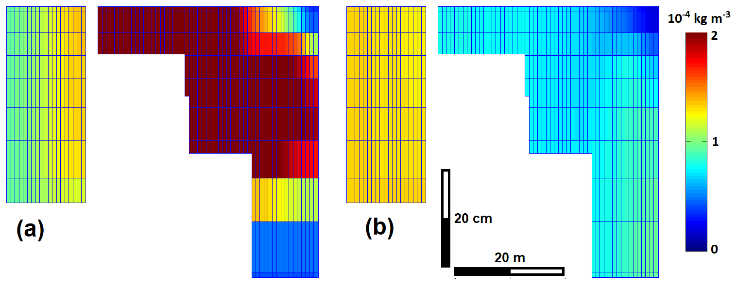
Figure 4 Tracer concentration on the longitudinal cross-section of Fig. 1a, for a tracing simulation with a constant flow rate, 17 h (a) and 41 h (b) after injection.

4 Discussion and conclusions

4.1 Quality of the wetland hydrodynamic model

The agreement of three-dimensional simulation with observations was satisfactory, in line with results reported for a laboratory tank (Adamsson et al., 2005). The detailed representation of vegetation contributes to the modelling agreement with observations (Bulat et al., 2019). While vegetation was homogeneous at the construction, its evolution over time can create preferential flow paths which degrade the hydraulic efficiency, here the short-circuit index. The seasonal evolution of vegetation should also be taken into account in a simulation over several months.

4.2 Effect of the flow rate on the hydraulic performance

Results showed that short-circuit index and the dimensionless mean residence time increase slightly with the flow rate whereas the mixing index remains stable, which is consistent with the experimental results of Holland et al. (2004). When, the flow rate is greater than 40 L s⁻¹, the dimensionless mean residence time exceeds 1, which is not possible when using 2D simulation models (Persson et al., 1999).

To explain this behavior, we can observe in the longitudinal cross-section (see Fig. 1a) that the tracer can remain partly stored deeply in the 1st compartment of the wetland, even almost two days after the injection (Fig. 4b). Since the inflow comes from agricultural subsurface drains through soil profile, its temperature is quasi constant, whereas water temperature follows the dynamics of air temperature and sunlight. A cold inflow during tracer injection plunged to the depth where wetland water had the same temperature. Later, a warmer inflow remained close to the surface (Peeters and Kipfer, 2009). In such a stratified flow, the mean residence time can be higher than the theoretical residence time.

The results of this study show that, in wetlands with a controlled water level, a tracing at low flow provides reliable information about the average hydraulic performance, especially the mean residence time and mixing which are of major interest for treatment. This is all the more interesting since environmental tracings require quasi steady flow conditions and UAV observations in good weather conditions. Periods of several days of both relatively stable high flow and good weather are rare.

Holland et al. (2004) showed that water depth has a greater influence on hydraulic performance than the flow rate. Thus, if the management allows regulation of the water height, its variations have to be considered in an annual (or multiannual) assessment.