GNSS measurements for ground deformations detection around offshore natural gas fields in the Northern Adriatic Region

The study aims to evaluate ground deformations in a vast area characterized by the coexistence of intense anthropic activities and offshore natural gas production. Onshore subsidence can be studied by GNSS, InSAR, high precision leveling and extensometers that provide broad datasets for a fully integrated description of the phenomenon. At present, seafloor subsidence monitoring cannot be carried out by high precision leveling, and GNSS is the only reliable method, implemented by means of permanent stations installed on offshore hydrocarbon production facilities. In the Northern/Central Adriatic Sea gas production platforms, GNSS data are recorded since more than 15 years, allowing to estimate not only the average subsidence of the platform/seafloor, but also possible velocity variations due to underground fluids withdrawal. This study shows the comparison of 22 offshore GNSS permanent stations located in the study area. Raw data have been processed with two different software packages (GIPSY-OASIS and GAMIT-GLOBK) based on different approaches and considering different boundary conditions of geodetic and/or modeling nature. Main results point out the high accuracy of the GNSS technology considering also the impact of data processing. Finally, at selected permanent stations we also performed a comparison of results obtained by GNSS, InSAR and high precision leveling.

1 Introduction

The Italian section of the northern Adriatic Sea is a vast area characterized by the presence of many natural gas production fields, located both onshore and offshore, or straddled in between the shoreline. The altimetry and the geological features of the coastal area make it very sensitive to flooding. This territory encompasses the Eastern part of the Po Valley sedimentary basin, which is characterized by Pleistocenic unconsolidated deltaic sediments. Here, large areas are located at about the mean sea level, or even below. Moreover, the coastal lowlands and deltaic plains of the Emilia-Romagna and Veneto Regions, including the Po River delta, are historically affected by relevant subsidence phenomena, which includes also many inland areas of the Po Valley, such as the plain areas surrounding the highly populated urban areas of Bologna, Modena, etc. (Brighenti et al., 1995; Teatini et al., 2005). Therefore, in these areas it is paramount to monitor both the natural subsidence of the recent sediments and the eustatic variation of the mean sea level, and to limit as much as possible the anthropogenic subsidence due to underground fluid withdrawal. In some cases, land subsidence and other natural phenomena have been associated with anthropic activities, such as natural gas production and intense aquifer exploitation, making subsidence a hot topic in the public debate. Therefore, a strong effort is carried out in order to guarantee an effective monitoring of the territory, in terms of subsidence rates, especially in those areas close to production fields.

At present, several monitoring techniques are available for vertical displacements monitoring, such as high precision leveling, GNSS (Global Navigation Satellite Systems) and InSAR (Interferometric Synthetic Aperture Radar). In particular, high precision leveling is very accurate and reliable, with an accuracy in the order of 1 mm km⁻¹, although it only provides a discrete description of the height variations and is quite expensive for the monitoring of large areas.

Differently, InSAR techniques have the advantage of providing virtually continuous datasets (interferograms) with an accuracy of a few mm. For this reason, despite the high cost of data processing, InSAR techniques can be considered a cost-effective alternative to high precision leveling whenever large areas must be monitored. Unfortunately, both high precision leveling and InSAR cannot be easily applied in offshore environments, due to the impossibility of using leveling instruments in the marine environment and because of the poor reliability of InSAR interferograms estimated on small stable spots surrounded by the incoherent shapes of the sea waves.

At present, GNSS give the estimation of the ellipsoidal vertical coordinate with centimetric level of accuracy. Nevertheless, its capability of producing continuous data acquisition provides very consistent time series that, if properly analysed, leads to estimations of velocity trends with mm per year level of accuracy. GNSS receivers can be easily installed on offshore structures and therefore this technique is becoming an important tool for the subsidence monitoring of hydrocarbon production areas. Actually, novel techniques for offshore seafloor subsidence monitoring are under development, but not yet operative on a large scale (Miandro et al., 2017; Cenni et al., 2017).

The present paper focuses on the impact of different calculation approaches and different software packages for GNSS data processing on the estimation of time series trends. A test was performed based on a consistent dataset of GNSS data gathered by 34 permanent stations, 12 located onshore and 22 installed on offshore gas production structures for a period of about seven years (Fig. 1). Two different calculation approaches have been considered, the classical relative approach performed using the GAMIT-GLOBK (Herring et al., 2015) and the PPP (Precise Point Positioning) approach implemented in the GipsyX software packages (Webb and Zumberge, 1997). Finally, the paper compares the estimation of subsidence velocity by using the three abovementioned techniques on a particular case study in the investigated area (Northern Adriatic Region), in the same timeframe.

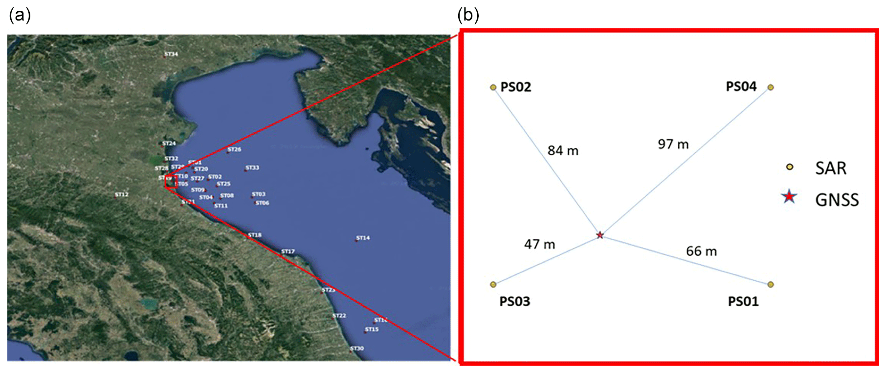
Figure 1 General map of the investigated area. (a) map of the investigated GNSS permanent stations (Map data © Google 2019). (b) relative position of the four InSAR persistent scatterers (PS1, PS2, PS3 and PS4) with respect to the ST19 GNSS station.

2 Impact of different GNSS data processing approaches in offshore subsidence monitoring

The dataset analysed in this study is constituted by daily RINEX (Receiver Independent Exchange format) files provided by 34 GNSS permanent stations located along the Emilia-Romagna coastline (12 onshore stations) and in the north-west Adriatic Sea (22 offshore stations). GNSS observables were acquired with 30 s interval from 2007 to 2013. The whole dataset was processed using both the GipsyX and the GAMIT-GLOBK software packages. The first one is the latest release of the GIPSY-OASIS software, developed and maintained by the NASA Jet Propulsion Laboratory, which implements a PPP approach. Therefore, it has the capability to provide highly precise coordinates of a single receiver using both code and carrier phase observables (Gandolfi et al., 2016). Conversely, the GAMIT-GLOBK software package, developed at Massachusetts Institute of Technology, implements the classical differenced approach toward the GNSS observables, thus providing the estimations of the baseline vectors linking two or more receivers. The boundary conditions used for the data processing were as much as possible the same for both software packages. In particular, VMF1 tropospheric mapping function (Herring et al., 2008) and igs_14.atx absolute antenna calibration files were used. Moreover, all the coordinates' solutions were aligned to the ITRF2014 reference frame using Helmert transformation parameters estimated ad hoc by using the same 9 International GNSS Service reference stations.

As for the post processing of the coordinate solutions, both datasets were treated using the same automated procedure that, basing on the Least Squares approach and the Heaviside function, allows to solve discontinuities in time series and to estimate the mean velocity parameters. The mean velocity of the height component characterizes the subsidence trend over the considered period. Aim of the test was to assess the coherence between the solutions given by the two different calculation approaches. Table 1 reports the differences between the velocity estimations calculated by the two abovementioned software packages, together with the related uncertainties, which were calculated by applying variance propagation.

Table 1 Columns Δv_u and σ_Δvu report the difference between the mean vertical velocities (mm yr⁻¹) estimated by using two different software packages and the related uncertainties, calculated by applying a variance propagation. The stations showing a statistically significant inconsistency are highlighted. Only true differences are reported for confidentiality reasons (data provided by Eni S.p.A.).

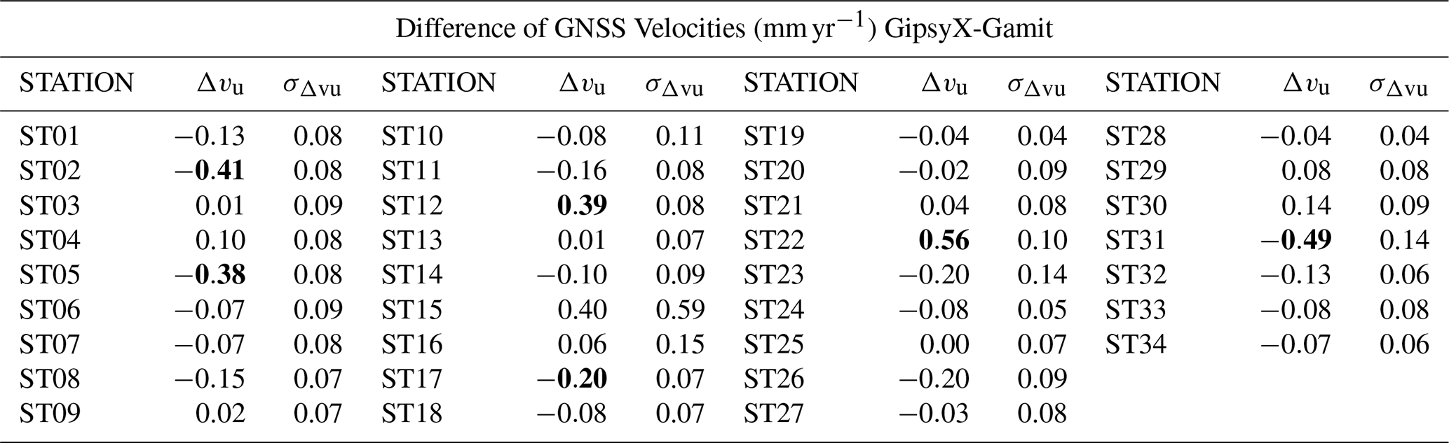
Results show a consistency of about 0.1 mm yr⁻¹ for most of the GNSS stations, with a few cases up to 0.5 mm yr⁻¹. Figure 2 shows the Up component of one of the investigated GNSS station calculated by the two software packages. From a statistical point of view, assuming a 3-sigma confidence interval, there are only five stations showing significantly different vertical velocities, highlighted in Table 1. Nevertheless, it should be stressed that the maximum of these differences has a magnitude of 0.6 mm yr⁻¹, which is actually at the limits of the GNSS technique sensitivity, and the statistical significance of these differences is mostly due to the very small uncertainties that characterize the time series. Being the mean velocities calculated using the two different software not significantly biased, in the following a combination of the two solutions is considered as the GNSS estimation of the subsidence trends. This combination was calculated by computing the average values between the two solutions for each day, weighting these by the inverse of their formal error.

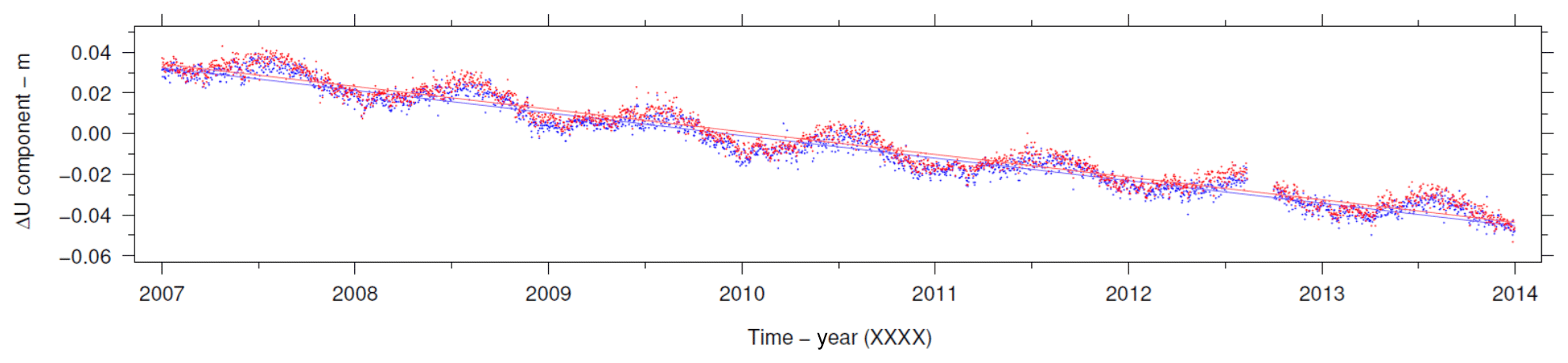
Figure 2 Example of the time series of the Up coordinate component in a selected station in the investigated area. Values have been calculated by using GipsyX (blue dots) and GAMIT (red dots) software. Coordinates are referred to a local topocentric reference and are expressed in m. Regression straight lines are superimposed to the correspondent time series.

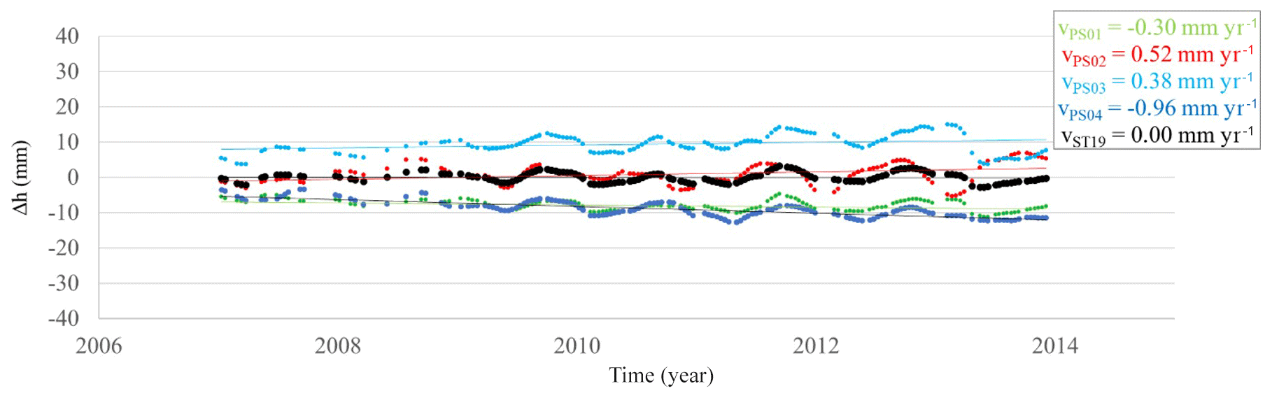
Figure 3 Time series of the InSAR measurements for PS1, PS2, PS3 and PS4, plotted together with the related regression straight lines. Black dots represent the combined values in correspondence of ST19 GNSS station19. The regression straight line has been assumed as reference for data confidentiality reasons.

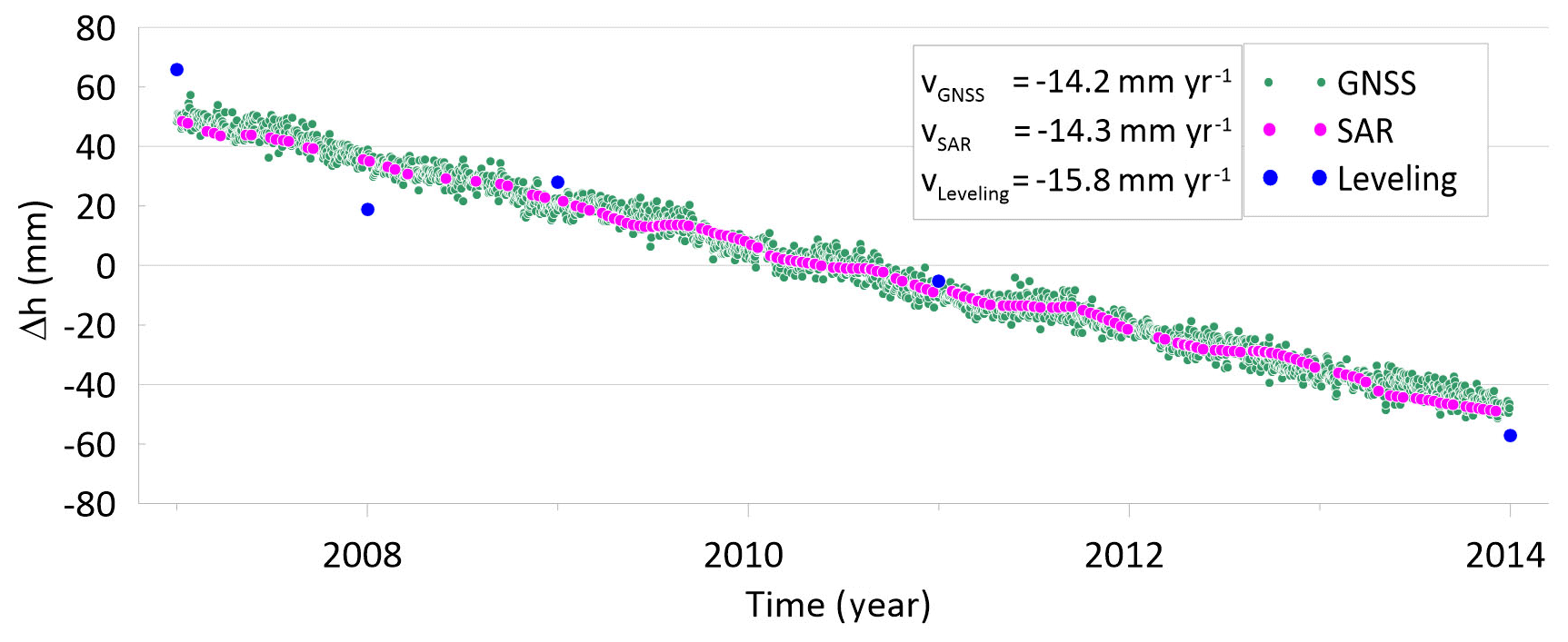
Figure 4 Residual time series with respect to the GNSS velocity of the vertical coordinates measurements using InSAR (purple dots), GNSS at ST19 GNSS station (green dots) and high precision leveling (blue dots).

3 Comparison between different onshore subsidence monitoring techniques

A comparison between the vertical velocities estimated using different techniques is here discussed. About 9 m far from the permanent station ST19 a levelling benchmark is present, and therefore this site has been chosen for the comparison. Moreover, data from five high precision leveling surveys are available in the considered period, which were performed starting from a benchmark close to ST34, which is located approximately 160 km north of ST19. The hypothesis of vertical stability of ST34 is assumed in the estimation of the trend derived from such data. It was thus necessary to subtract the vertical velocity of ST34 from the one of ST19 in order to make the GNSS trend estimation comparable to the one derived from high precision leveling. As for the InSAR data, four persistent scatterers (PS), with the related time series, were available close to the ST19 site. Location and distances between the PSs and the GNSS station are shown in Fig. 1. InSAR data where acquired by the RADARSAT 2 satellite and processed by e-GEOS using the PSP-DIFSAR technique. This technique allows, basing on both ascending and descending satellite orbits, to estimate position variations along the vertical direction. In order to compute the InSAR estimation of the vertical trend to be compared with the ones derived from GNSS and leveling, the velocities given by the four PS (PS1, PS2, PS3 and PS4) were combined weighting each one by the inverse of the distance between the PS and ST19. The result of this combination is the time series reported in Fig. 3, which uses its regression straight line as reference. Figure 3 also shows the InSAR time series related to the abovementioned 4 PS, expressed relatively to the combined mean solution, and referred to ST19. The InSAR dataset available for this study has not been calibrated, and so all the measurements are referred to a single PS supposed to be stable in time, which is unknown. This fact introduces a bias in terms of velocities depending on the motion of the reference PS. In order to estimate such bias, the only possibility was to compute the averaged difference of vertical velocity for those sites where a GNSS station and a PS where co-located. In particular, this was possible for the sites ST05, ST28 and ST29 and the calculated bias was subtracted to the interpolated value estimated for the InSAR technique in ST19 position. Also in this case, the GNSS velocities calculation takes into account the subtraction of ST34 velocity values, and therefore the calculated InSAR velocity is fully comparable with the high precision leveling results. Fig. 4 reports the time series of the measurements performed with InSAR, GNSS and high precision leveling, all expressed with respect to the regression straight line calculated for the GNSS data. The three techniques lead to slightly different results, which are very similar for GNSS and InSAR, whereas the high precision levelling provides a difference of about 1.5 mm yr⁻¹. This can be explained considering both the high numerosity of the data sample and because InSAR technique is calibrated using GNSS data. Moreover, the error propagation of the leveling error is affected by the long distance of the starting benchmark, which is located about 150 km far away.

4 Conclusions

This paper investigates two main technical aspects concerning the estimation of the subsidence trends basing on geomatics surveys.

The first one relates to the impact of using different calculations approaches for the GNSS data processing, and thus also for different software packages. The two tested approaches are the commonly used relative approach and the Precise Point Positioning, implemented in the GAMIT-GLOBK and the GipsyX software packages, respectively. The test shows that, with the same boundary conditions, the two approaches leads to highly comparable results, at least while considering a robust dataset as the one considered here (seven years time series).

The second aspect concerns the consistency of the vertical trends estimated using different survey techniques, namely the classical high precision leveling, the GNSS permanent stations and the recently developed InSAR. This comparison has been performed on a site where survey data were available for all the three different techniques. The results show absence of discrepancies between InSAR and GNSS, by considering an accuracy of 0.1 mm yr⁻¹. The high precision levelling, which is affected by a significantly smaller data sample, has proved to be consistent with the other techniques considering within 1.5 mm yr⁻¹. This difference might have been lower by using a higher number of measurements and/or a closer reference benchmark. This test confirmed that, with sufficiently long datasets, all the considered survey methods can be used, choosing a specific one according to its strengths and limitations. InSAR is the choice to monitoring wide areas, whereas high precision leveling is still an efficient alternative for the monitoring of single objects, especially if not far away from a stable benchmark. Finally, the GNSS technique has proven to be a reliable tool and, at present, is the only one suitable for offshore applications.