the Creative Commons Attribution 4.0 License.
the Creative Commons Attribution 4.0 License.
 | 22 Apr 2020
On the uncertainties of monitoring subsidence from small sources: Dutch mining regulation on subsidence monitoring and its role in communication and accountability
Mathijs W. Schouten
Johannes A. de Waal
Mining induced subsidence in the Netherlands is often associated with small gas fields (less than 5 km diameter), or discrete sources (converging salt caverns). As most of the areas experiencing this subsidence are close to sea level, and the effects of gas exploitation in Groningen may be considered a national trauma, there is strong emphasis on control and regulation of the related mining activities and their effects at the surface. The relatively small subsidence (often less than 10 cm), combined with inherent prediction uncertainty involving geological parameters, introduces a monitoring challenge to both mining companies and the regulator. A large initial uncertainty can be reduced during production by a carefully designed monitoring strategy, including evaluation of the results and clear communication on the effects on the uncertainty of the prognosis. In the same process, one may quantify remaining uncertainties and the limitations on predictability. In this contribution, we discuss the nature of some specific uncertainties associated with small source subsidence, and the effects on the regulatory process. The description is based on a realistic assessment of the expected accuracy of subsidence predictions. This allows for a clean comparison between different measurement techniques, and may help prevent overly optimistic claims on predictability. A description of uncertainty in terms of scenarios and parameter sensitivity studies should be used in communicating the expected level of subsidence control to water management boards and the general public.
- Article
(1164 KB) - Full-text XML
- BibTeX
- EndNote


Mining and mining induced subsidence in the Netherlands is often first associated with the Groningen gas field, a large area where as much as 50 cm total subsidence is expected. In addition to the primary effects of subsidence in the gas field there are secondary effects that are equally important. These secondary effects include the effects on water management, agricultural qualities of the land, and the way people perceive mining as an activity that acts to deteriorate their living environment.
More than two hundred gas fields under the Dutch soil have been, or are currently being exploited (see Fig. 1). A set of regulatory activities are being implemented that focus on quality of prediction, monitoring and control of the induced ground movement (primarily subsidence). Additionally, salt mining activities in the northwest, northeast, and east of the country cause the most concentrated areas of subsidence, with decimetres movement, in rather isolated patches with strong gradients, often in areas that are also near active gas fields.
Here, we discuss some of the specific difficulties of predicting and monitoring subsidence caused by small or discrete sources. We keep in mind the purpose of regulation, which is to assure a balance of technical control, and establishing reliability and perception of control on the effects of mining activities. The latter are expressed by realistic uncertainties on any prediction given.
We show that an assessment leading to a large initial uncertainty is not necessarily problematic, when periodic evaluations and measurements are used to update the assessment and constrain the uncertainty of the effects for the near future within smaller bandwidths.
2.1 Small fields?
Only one of the currently producing gas fields in the Netherlands, the Groningen field, is officially called “not small”. All the other fields are considered “small fields”. If we summarize the extent of these fields by an effective radius, which is here defined as the radius of a circular area that covers the same area as the outline of the field, we get the picture shown in Fig. 2.

Figure 1Gas fields in the Netherlands.
The bulk of these fields has a radius of around 1–2 km, which corresponds to about 5 square kilometre in areal extent. People living near these fields often feel treated without the proper respect when policy makers refer to a field as “small” while they consider it a potential threat to their property or quality of life. The naming therefore is not particularly well chosen.
Here, what we call a small source is a field that has a spatial extent (represented by its effective radius Reff) smaller than or comparable to its depth (d). For the Netherlands, that would qualify indeed almost all fields except Groningen and perhaps some of the larger Wadden Sea fields. The relation Reff<d is clearly met for these fields, mostly located at depths of 2–3 km.
2.2 Discrete sources
Salt mining in the Netherlands is done by solution mining. This implies that caverns are created by flushing fresh water inside a layer of rock salt. The subsidence effects are usually modelled as discrete sources, located at the centre of the cavern location. Subsidence occurs when salt flow towards the cavern is induced by lower pressure than the lithostatic gradient outside. The single-source modelling is justified by the small effective radius of the area affected by the salt flow. This radius is in the order of a few hundred meters, so Reff≪d.
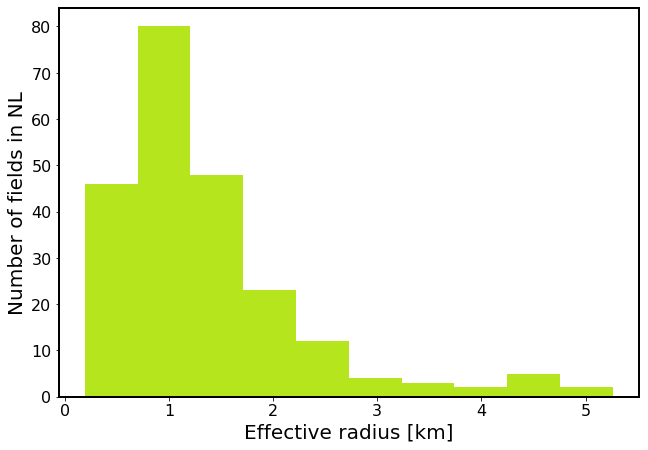
Figure 2Distribution of the size of the gas fields in the Netherlands, portrayed by their effective radius. With common reservoir depths of 2–3 km, the bulk of the fields are sized well below twice their depth.
3.1 An estimate of compaction
Any subsidence prognosis begins with an assessment of the field and the proposed gas production from that field in the case of gas production, or of the salt layer and squeeze characteristics in the case of salt solution mining. For salt squeeze towards a cavern, the volume loss is usually modelled at a single central location, where the total squeeze is concentrated. With squeeze diminishing quickly within the first few hundred meters from the pressure sink (the cavern), this is usually justified by the same Reff<d relation mentioned above.
The compaction expected in a gas reservoir is derived from the pressure depletion in the reservoir (ΔP), the geometry, and the visco-elastic characteristics of the reservoir material. In many cases, a simple one-dimensional relation for the vertical compaction (C) is used:
where H is the height of the reservoir, and Cm is a dimensionless compaction coefficient for compaction per bar of pressure depletion. This coefficient is typically valued between 10−7 and 10−4. The vertical compaction C is then the difference in height of the reservoir between the start of production and when the effects caused by production have equilibrated with ΔP. With these values, a 100 m thick reservoir, experiencing 100 bar of pressure depletion would experience between 1 mm and 10 cm of (vertical) compaction.
3.2 Compaction to subsidence
The translation from compaction at reservoir depth to subsidence at the surface is, either explicitly or implicitly, a spatial convolution. The compaction at reservoir depth is convoluted with a response (Green's) function that can often be characterized by a one-dimensional profile. This profile characterizes the result of a unit compaction at the depth of the reservoir, as a function of the distance from the projection to the surface (e.g. van Thienen-Visser and Fokker, 2017).
3.3 Horizontal homogeneity
Horizontal heterogeneities in the overburden are usually not modelled. Orlic and Wassing (2013) show subtle effects that arise from subsurface conditions deviating from ideal horizontally layered (a layer cake) conditions. Also, an investigation into the effect of a strong gradient in the thickness of a viscous salt layer by Pluymaekers et al. (2018) showed very little effect even for a rather extreme horizontal inhomogeneity. Here, we assume horizontal homogeneity. Also, a linear scale dependence of the one-dimensional profile of the subsidence due to a unit of compaction with the depth of the reservoir is often assumed. Such dependence is a characteristic of modelling approaches that consider a single depth for the reservoir. An excellent overview of these and other methods of forward subsidence modelling is given in van Thienen-Visser and Fokker (2017).
3.4 All volume accounted for
A common starting point for subsidence modelling is the assumption that all subsurface volume lost at depth, is found somewhere as subsidence at the surface. Deviations from this one-to-one match are usually attributed to temporal effects in the compaction or inadequacies of the volume measurement at the surface. Such measurements are intrinsically difficult, as a large part of the total volume is found at larger distance from the centre of the subsidence bowl: small movements over large areas can represent a considerable volume, while being hard to measure with the precision needed to confirm a one-to-one match with the compaction volume. The compacting volume is itself not often known with an accuracy.
3.5 Delayed response
These are several known causes for delays in the response of surface deformation to mining activities. These delays can arise from either the pressure adjustment, the compaction response to pressure depletion, or translation between reservoir depth and the surface. A summary of effects investigated in the scope of the Dutch Wadden Sea is given in de Waal and Schouten (this issue).
In the remainder of this contribution, we discuss some of the difficulties in discriminating a temporal delay from uncertainties in the determining the eventual total subsidence caused by small or discrete sources.
4.1 Size of field determines deepest point subsidence
Depending on the width of the influence function, the size of the compacting reservoir determines not only the areal extent of subsidence at the surface, but also the amplitude. For a large field (Reff≫d) 10 cm of reservoir compaction yields 10 cm of subsidence, and the influence function determines only the shape of the profile at the field edge. However, when the gas field is smaller than the surface footprint of a single nucleus of strain or point-source compaction contribution, the maximum subsidence is smaller than the compaction at reservoir depth. How much smaller, depends both on the influence function and on the size of the field.
In Fig. 3, we show for a circular uniformly compacting reservoir and a given influence function, the shape of the subsidence response between the centre of the bowl and the unaffected periphery. The profiles are centred at the edge of the field, and normalized by the depth of the reservoir and the compaction at reservoir depth.
The profile itself is based on a Geertsma (1966) and van Opstal (1974) solution with a rigid basement form-factor of 1.4 times the depth of the reservoir. For field radii between 0.3 and 2.5 times the depth of the field, the subsidence in the middle of the bowl increases from a mere 15 % to about almost 100 % of the field compaction. A similar plot for a profile with a rigid-basement form-factor of 1.1 (resulting in a smaller but steeper bowl) gives similar values between 20 % and 100 % for similar values of field radius to depth ratios (Fig. 4).
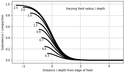
Figure 3For various relevant field radius ∕ depth ratios (plotted to the left of each line) the subsidence profile between the centre of the resulting bowl (centred at the edge of the field), show how for smaller fields, the maximum subsidence is only a fraction of the compaction at reservoir depth. The subsidence effects are minimal at 1–2 depths distance from the field edge.
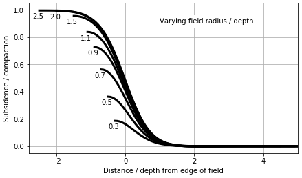
Figure 4As Fig. 3, but for a steeper bowl form factor. Due to the now smaller surface expression of a point source, fields larger than twice the depth will see the full compaction as subsidence.
4.2 Profile determines depth of deepest point
As was clear from the comparison between Figs. 3 and 4, the shape of the profile (and thereby the overburden properties and modelling approach chosen) for smaller fields strongly affect the total subsidence. The difference between a small and a larger field is illustrated in Fig. 5, where for a larger field (a radius of 3 times the depth) the profile only subtly changes the edge of the subsidence bowl (for a range of form factors), but for a smaller field (of comparable radius to reservoir depth) the same profiles determine where the maximum subsidence ends in a five-fold range between 0.1 and 0.5 times the compaction at reservoir depth.
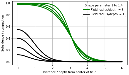
Figure 5For a smaller field (black lines), the choice of the one-dimensional profile strongly determines the maximum subsidence, whereas in the case of a large field the profile only affects the gradients ad the edge of the field (green).
Clearly, most gas fields in the Netherlands fall in the range where the total subsidence is strongly affected by the size and shape of the field. This leads to a mixed effect of reservoir properties (the Cm value in the simplest expressions) and overburden properties (which determine the steepness of the profile).
As for small fields or discrete sources of subsidence the total subsidence expected for a given pressure depletion is clearly hard to predict within a narrow bandwidth, time dependent effects (a delay in subsidence) may initially be misinterpreted as indications of smaller than expected compaction. When such interpretations are used to adjust an initial prognosis, one may later have to return to an original – often higher – subsidence prognosis. This strongly reduces the reliability and (over time) the credibility of subsidence predictions. It adversely affects the public confidence in the level of control by the operator and the regulatory bodies.
Here, we provide a simple example to illustrate the mixed effect of uncertainty in both the delayed response of subsidence, and in the total amount of subsidence that will eventually occur, and which we have seen to be difficult to assess beforehand, even with good knowledge of the reservoir characteristics. We model a simple square reservoir sized 4×4 km, located at a depth of 2.5 km, yielding a ratio Reff∕d of just over 2. The “true” reservoir compaction amounts to just over 20 cm, for ΔP=200 bar, H=40 m and . The reservoir compaction has a temporal delay modelled by a 2 year decay scale. The reservoir depletion occurs over a production period of 20 years.
We use this scenario, and an initial uncertainty in the important parameters of total subsidence and time decay, to investigate the effects of measurements in reducing the initial uncertainty. As measurements, we consider a single observation point in the middle of the subsidence bowl. Measurements away from the centre might help determine the profile, but we have seen that there is little sensitivity of the profile on the flanks of the bowl, and measurements may not be accurate enough to reduce an initial uncertainty here.
The initial combined uncertainty in terms of the total subsidence in the middle of the resulting bowl summarizes the effects of H, Cm, and characteristics of the over- and underburden through the 1D profile (or the form factor), is modelled by varying the estimate of Cm between and . The initial uncertainty in time-dependence is modelled by a time decay coefficient between 0 (for immediate response) and 5 years. The initial uncertainty at the start of production is modelled through an ensemble of possible scenarios, all of which are somewhat likely. In Fig. 6, we show the complete ensemble of possible outcomes for a period of 30 years, which is 10 years longer than the period of production. The time lag uncertainty yields several paths towards the same total deformation values. This rather large range of uncertainty yields a mean (“estimated”) value of 25 cm subsidence.

Figure 6The a priori ensemble of possible subsidence scenarios (green lines), given an initial uncertainty in the value of the deepest point, and in the time path towards this value (given different values for a possible time-delay coefficient). The “true” scenario is plotted as an orange dashed line, the mean of the ensemble (or best a priori estimate) as a black line.
During production, subsidence measurements (n) are made at the centre of the bowl, at fixed intervals of five years. We show in Fig. 7 the resulting range of scenarios fitting the measurements as green, with the initial bandwith in grey to illustrate the increase in predictive confidence, that is achieved by making the measurements. We will not go into the exact ways of selecting the likely scenarios, but suffice to mention the measurement accuracy which can be used to value the likelihood of each member, and a 90 % confidence band, which is chosen to contain the 90 % of likeliness-weighted members of the initial ensemble.
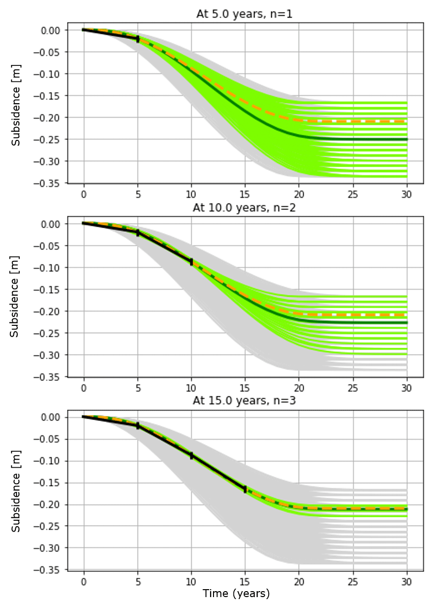
Figure 7At five-year intervals, measurements in the deepest point of the subsidence bowl are used to constrain the initial ensemble (grey) to a 90 % confidence band (green) and a new weighted estimate of the future subsidence (black line).
After five years, this yields a measurement in full agreement with the prediction, but without any predictive power, in the sense that the full range of possible outcomes is still possible: with a single measurement, some of the more extreme scenarios are discarded (now colored gray in Fig. 7), but there is no way of knowing whether the deformation has been delayed and headed towards a larger value, or more immediate and headed towards less subsidence.
After the second measurement (n=2) at ten years (and note that we are already halfway through the 20 year production period) the bandwidth of likely scenarios begins to narrow, and the total subsidence estimate is adjusted towards the “true” value. At n=3, fifteen years into production (third panel of Fig. 7) the uncertainty range is strongly reduced. Now that about 80 % of the production is in the past, and peak production is also some time ago, the measurement leads to a strong improvement in the estimate of the final 25 % of the subsidence.
One way to reduce the uncertainty earlier, measuring more often, only slightly helps to reduce the bandwidth. In Fig. 8, we show the equivalent of the middle panel in Fig. 7 at ten years, but now for measurements acquired every 2.5 years, thus n=4. The resulting bandwidth is very similar to that in Fig. 7 at ten years.
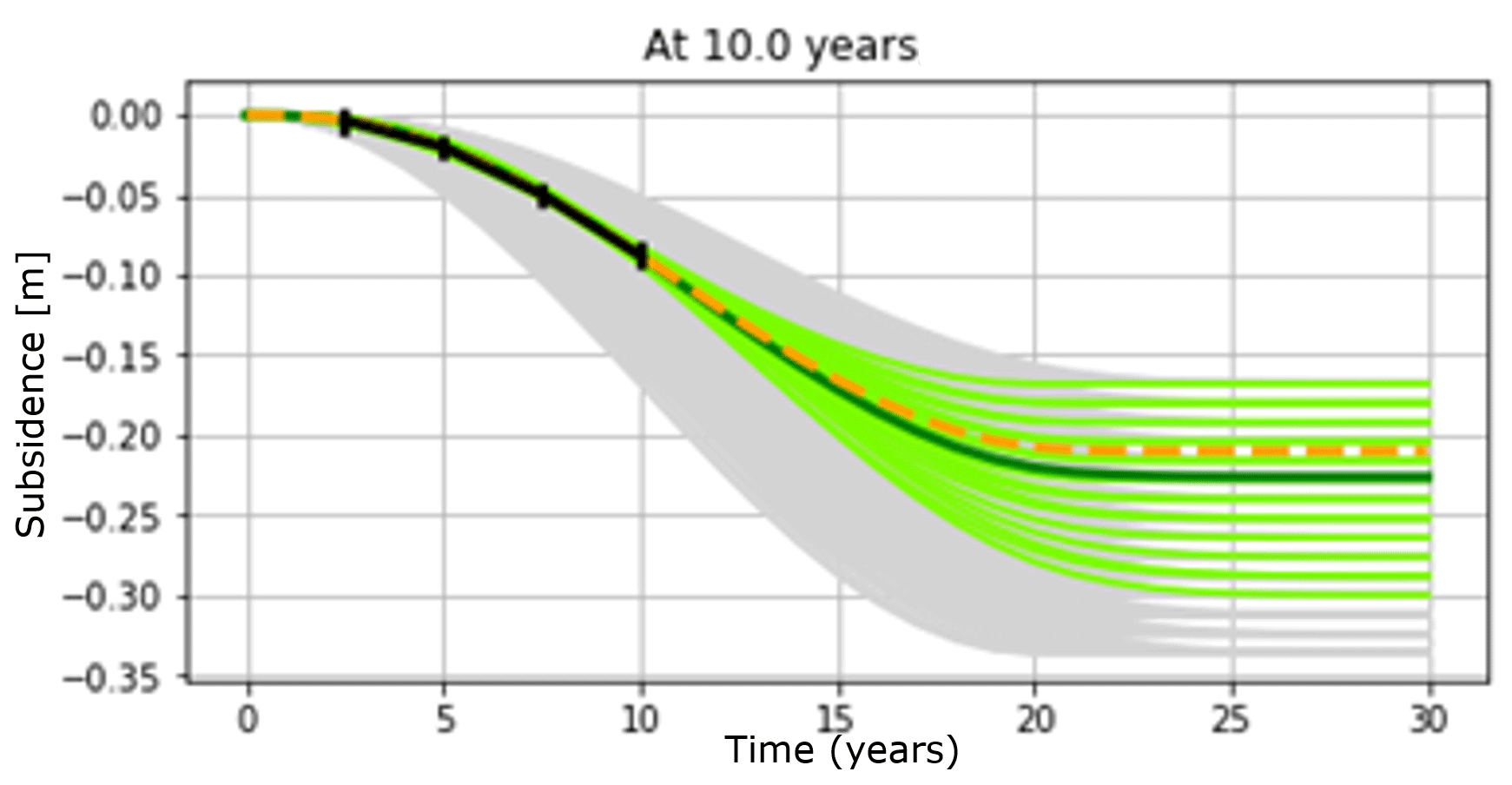
Figure 8As the middle panel of Fig. 7, but now for more frequent measurements, taken every 2.5 years.
At the State Supervision of Mining (SSM) in the Netherlands, we exercise the Dutch mining laws and regulations, which state that a prognosis of effects at the surface must be determined before operations can be allowed. This prognosis includes an assessment of its uncertainty. Ministerial consent with these prognosed effects is given after consulting the local water management boards, municipalities and technical advisors.
During production the mining operator periodically measures the effects (the most visible of which is subsidence), to ensure that operations are within the predicted bandwidths. With uncertainty being inherently large (in relative terms at least – in absolute terms, for most gas fields in the Netherlands the uncertainty is well below 5 cm) it is not immediately clear when regulatory actions are required. What is “the prediction” to compare with measurements, and when is a measurement no longer in agreement with prognosed effects? These questions require a proper description of uncertainties in both the prognosis and the measurements.
That said, the uncertainty in measurements is not to be ignored, but also not to be exaggerated: compared to the uncertainty in a priori modelling, the measurements are rather exact. Levelling in a well-designed network results in standard deviations for individual benchmarks that are often well below the 1 cm level. Especially for these smaller fields, a 1 cm deviation measured over a substantial area is a signal that cannot be ignored as “possible measurement error”.
The modelling of subsidence, on the other hand, involves assumptions that are realistically inaccurate on another scale. This involves uncertainties that can easily exceed the cm level. This realisation may lead to descriptions of a “high case” that is conservative in many ways, and describes an edge case that is unlikely to occur. Based on this “high case” prognosis of the effects, local governments plan their remedial works (if necessary).
Dealing with the large uncertainty in a prediction, leads to questions as to the proportionality of preventive measures. For example, how realistic is the case illustrated in Sect. 5, where local governments may start preparations for almost 35 cm of subsidence in year 1, when for all scenario's evaluated this effect may not be realized for another fifteen years or more, during which many other things may happen? In the remainder of this contribution, we discuss an alternative way of dealing with uncertainties on different timescales, and on ways to communicate these uncertainties to local authorities and the public.
7.1 Regulatory issues dealing with uncertainty
Given the large uncertainties of subsidence predictions due to production from small fields (in the case of gas) or discrete sources (in the case of salt solution mining), we propose to stimulate an open discussion of these uncertainties at the start of production. The nearly 35 cm maximum subsidence in the example in Sect. 5 should be mentioned as a possibility to local authorities, who can then investigate the measures required to deal with both the minimum and maximum effects.
However, the uncertainty on shorter timescales may be much smaller than that on the timescale associated with the full production lifetime of a field. In the example, the uncertainties in a five-year prediction are almost always less than 5 cm. At the start of production, one may ask whether it very likely that 5 cm subsidence will be reached after five years of production, or is this likely to happen anywhere between five and ten years from start of production? There is ample time to take the necessary management measures. At year 5, the prediction for year 10 is no longer the 5–18 cm wide range that it was at the beginning, but is now an 8–12 cm window (see Fig. 7). Also, it is now very likely that 15 cm will be reached within the next ten years, so management measures for an expected 15 cm of subsidence are appropriate at this point. After ten years, one may discuss several options: measure more frequently, or prepare for 25 cm of subsidence.
Shared knowledge about the large a priori uncertainty may thus avoid unnecessary investment in management measures for situations that may not occur. By implementation of a well-designed control cycle, management measures are taken when necessary and in due time. However, this requires somewhat more concertation between the mining operator, the regulatory bodies and local governments. This requires a degree of trust.
7.2 Communicating uncertainty
Once the effects deviate from those expected, the operation certainly deviates from planned operation. This implies a lack of control by both the operator and the government in its dual role as permit provider and supervisor. Not only is the prognosis and measurement cycle meant to keep the effects within a predefined acceptable range, it is also meant to maintain and demonstrate control over the operation.
Adjusting a prognosis should be avoided. Narrowing down a prognosis from a large initial uncertainty to a more focussed expected final outcome during production is explainable and transparent. A formal analysis step after doing periodic measurements can provide a good means of communication to the public and local governments. Interpretation of measurements in terms of reducing the uncertainties is often ignored, but may help explain how the effects of mining activities are kept under control.
One should avoid stimulating overly conservative prognoses meant only to seek permission for a larger operating range. In that case, the effects are exaggerated, and public concern and costs of mitigating measures for both the operator and the government may be raised beyond what is necessary.
The permitting process, and the associated planning and control cycle should incorporate the large initial uncertainty, but also provide reasonable limits on the shorter timescale, assuring timely measurements and evaluation of the impact of these measurements. Such a system can be used to find a balance between realistic assessment of what is known and what is not, and a cautious decision on measures and continued operation.
The uncertainties of total subsidence predictions from production out of small gas fields or discrete sources (of salt squeeze production) are large compared to the predicted subsidence itself, and also large when compared to the predictions for a large field, even with good knowledge of the field characteristics. Acknowledgement of these uncertainties is essential in maintaining public understanding of mining under a densely populated country near sea level. A well-designed and well communicated measurement and analysis cycle can help maintain control without excessive costs or unnecessary preventive measures.
The data are available at https://doi.org/10.17026/dans-2a9-2zkt (Schouten, 2020).
Both authors contributed in development of the ideas outlined in this paper. The simulations were performed by MWS. Both authors contributed to the text of the paper.
The authors declare that they have no conflict of interest.
This article is part of the special issue “TISOLS: the Tenth International Symposium On Land Subsidence – living with subsidence”. It is a result of the Tenth International Symposium on Land Subsidence, Delft, the Netherlands, 17–21 May 2021.
Geertsma, J.: Problems of Rock Mechanics in Petroleum Production Engineering; Proceedings 1st Congress of the International Society of Rock Mechanics, Lisbon, Vol. 1, 585–594, 1966.
Orlic, B. and Wassing, B. B. T.: A study of stress change and fault slip in producing gas reservoirs overlain by elastic and viscoelastic caprocks, Rock Mech. Rock Eng., 46, 421–435, 2013.
Pluymaekers, M., Breunese, J., Roholl, J., Pruiksma, J., and Orlic, B.: Langetermijneffecten van gaswinning op bodemdaling, TNO report R10859, 2018.
Schouten, Dr. Ir. M. W.: Analysis of subsidence resulting from small gasfield production in the Netherlands, DANS, https://doi.org/10.17026/dans-2a9-2zkt, 2020.
van Opstal, G. H. C.: The effect of base-rock rigidity on subsi-dence due to reservoir compaction, in: Proc. 3rd Congr. Int. Soc. Rock Mech., Vol. 2, 1102–1111, 1974.
van Thienen-Visser, K. and Fokker, P.: The future of subsidence modelling: Compaction and subsidence due to gas depletion of the Groningen gas field in the Netherlands, Neth. J. Geosci., 96, S105–S116, https://doi.org/10.1017/njg.2017.10, 2017.
- Abstract
- Introduction
- Small or discrete sources
- Characteristics of modelled subsidence
- Notable effects for small fields
- Unknown compaction and time dependence
- Control issues
- Consequences for regulation and communication
- Conclusions and recommendations
- Data availability
- Author contributions
- Competing interests
- Special issue statement
- References