the Creative Commons Attribution 4.0 License.
the Creative Commons Attribution 4.0 License.
 | 22 Apr 2020
Integrated monitoring of subsidence due to hydrocarbon production: consolidating the foundation
Gini Ketelaar
Hermann Bähr
Shizhuo Liu
Harry Piening
Wim van der Veen
Ramon Hanssen
Freek van Leijen
Hans van der Marel
Sami Samiei-Esfahany
This paper describes several geodetic studies that consolidate the reliability and precision of monitoring subsidence due to hydrocarbon production: the deployment of Integrated Geodetic Reference Stations (IGRS); the application of high resolution InSAR; the comparison of different GNSS processing methodologies; the implementation of an efficient InSAR stochastic model, and the framework of integrated geodetic processing (levelling, GNSS, InSAR). The advances that have been made are applicable for any other subsidence monitoring project.
- Article
(2214 KB) - Full-text XML
- BibTeX
- EndNote


Since the start of hydrocarbon production in the Netherlands, the Nederlandse Aardolie Maatschappij (NAM) has performed subsidence monitoring over its gas and oil fields, following Dutch legislation and the commitment to produce in a safe and responsible manner. Innovative geodetic acquisition techniques for subsidence monitoring (GPS/GNSS, InSAR) have been actively investigated and deployed over the past decades, as well as state-of-the-art processing and geodetic testing techniques. The solid foundation that has been established for subsidence monitoring has been reinforced towards the future by incorporating the latest (scientific) developments. This paper addresses recent results from the geodetic studies that are part of the production plan of the Groningen gas field:
-
The deployment of Integrated Geodetic Reference Stations (IGRS).
-
The application of high-resolution InSAR.
-
Improvement of the InSAR stochastic model.
-
Comparison of GNSS processing methodologies.
-
Integrated geodetic processing of levelling, GNSS and InSAR measurements (concept).
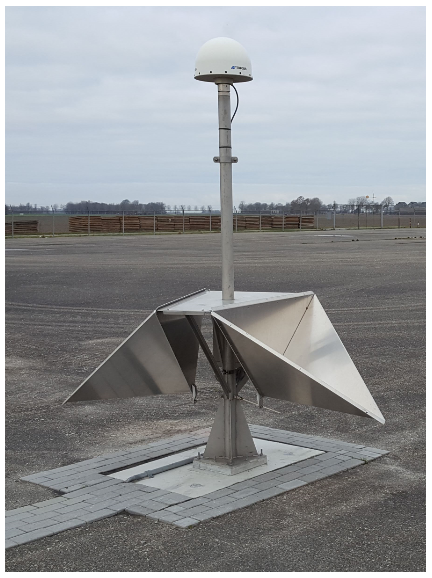
To further improve the subsidence monitoring network over the Groningen gas field, NAM has deployed 25 Integrated Geodetic Reference Stations (IGRS) since 2018 (Hanssen, 2017; Kamphuis, 2019). The IGRS consist of a GNSS receiver, two InSAR corner reflectors (for ascending and descending tracks) and several levelling benchmarks, all mounted on the same deeply founded monument (Fig. 1). The advantage of the IGRS is that the accuracy of levelling, GNSS and InSAR deformation estimates can be cross-validated directly, since the measurements are with respect to the same monument and hence reflect the same deformation cause. Also, spatially-dependent biases and noise can be assessed and mitigated.
The IGRS support minimizing subsurface uncertainties and optimizing future subsidence predictions. The density and location of the IGRS have been chosen such that the areas with the largest uncertainty in subsurface behaviour are captured (e.g. areas with potential aquifer depletion that do not contain wells). These areas are primarily located at the edge of the Groningen gas field, where horizontal movements are expected to be the largest. The IGRS target density was chosen such that the expected horizontal deformation signal can be reconstructed, considering the GNSS noise structure.
From the three geodetic techniques, only GNSS delivers all 3D deformation components (East, North, Height) with high precision. GNSS measurement precision (1σ) of the height component is 2 mm (Nederlandse Aardolie Maatschappij B.V., 2017), which implies that movements larger than 4 mm can be detected with 95 % confidence level. The precision of the horizontal components is slightly better.
Figure 2 depicts the latest analysis results of the vertical and horizontal movements of the Groningen IGRS. Based on geomechanical predictions, horizontal deformation rates are expected 0 in the center of the gas field, and ∼2 mm yr−1 at the edges of the field in the direction towards the center. All IGRS have been connected to the 2018 Northern Netherlands leveling campaign. IGRS InSAR time series processing will be performed in late 2019.
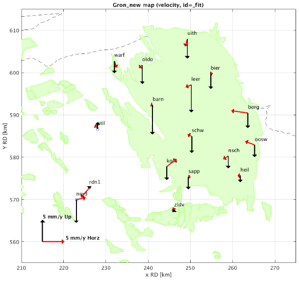
Figure 2Horizontal and vertical deformation in mm yr−1 for the IGRS that are operational more than 1 year, from start of deployment until mid 2019. The green areas depict the gas fields. The station “nor3” contains a fluctuating component due to gas injection and extraction.
Three TerraSAR-X tracks (two descending and one ascending) have been processed by SkyGeo B.V. for NAM covering the time period 2013–2019 (Qin et al., 2019). The high spatial and temporal resolution enables near-realtime building and infrastructure stability monitoring. Furthermore, a more detailed insight into horizontal movements is possible. However, due to the almost north–south oriented orbit, only the east–west component of the horizontal movements can be estimated well from the TerraSAR-X results. Figure 3 shows the horizontal movements over the Groningen gas field in the direction of the ascending look direction projected on the horizontal plane (almost east-west oriented, ∼10∘ angle). Also clearly visible is the horizontal deformation signal in the salt mining areas (near Veendam and Winschoten). The horizontal movements over the Groningen gas field in the recent year are as expected still below measurement precision; there is not yet a strong correlation with the IGRS processing results. However, the time series of the GNSS stations that have been operational from 2013/2014 have been cross-validated with the TerraSAR-X data (Line-of-Sight) and have shown agreement at millimeters level.
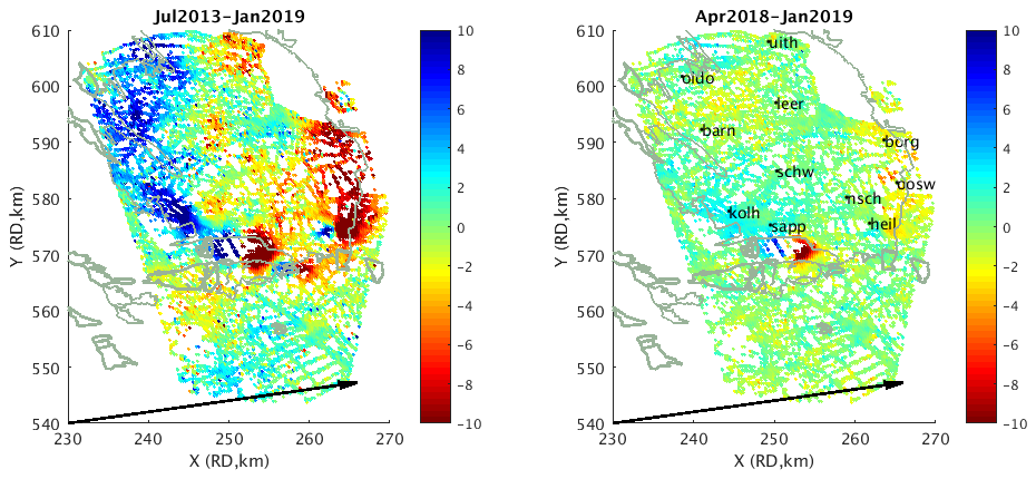
Figure 3Horizontal deformation (mm) in the direction of the ascending look direction projected on the horizontal plane (arrow) for the time periods 2013–2019 and 2018–2019, including the location of the IGRS that are operational minimal from April 2018. The outlines of the gas fields are depicted in grey.
The high-resolution InSAR processing results have also been used to investigate whether it is possible to discriminate between shallow and deep (at hydrocarbon reservoir level) deformation. Two methodologies can be used for this: separation based on the deformation histogram of neighbouring Persistent Scatterers (PS), and PS separation based on height above ground level. The latter turned out to be the most effective for high-resolution InSAR and has led for the first time to a localized clear shallow deformation pattern (up to 2 mm yr−1 rates) in Groningen that correlates with soil composition (Fig. 4).
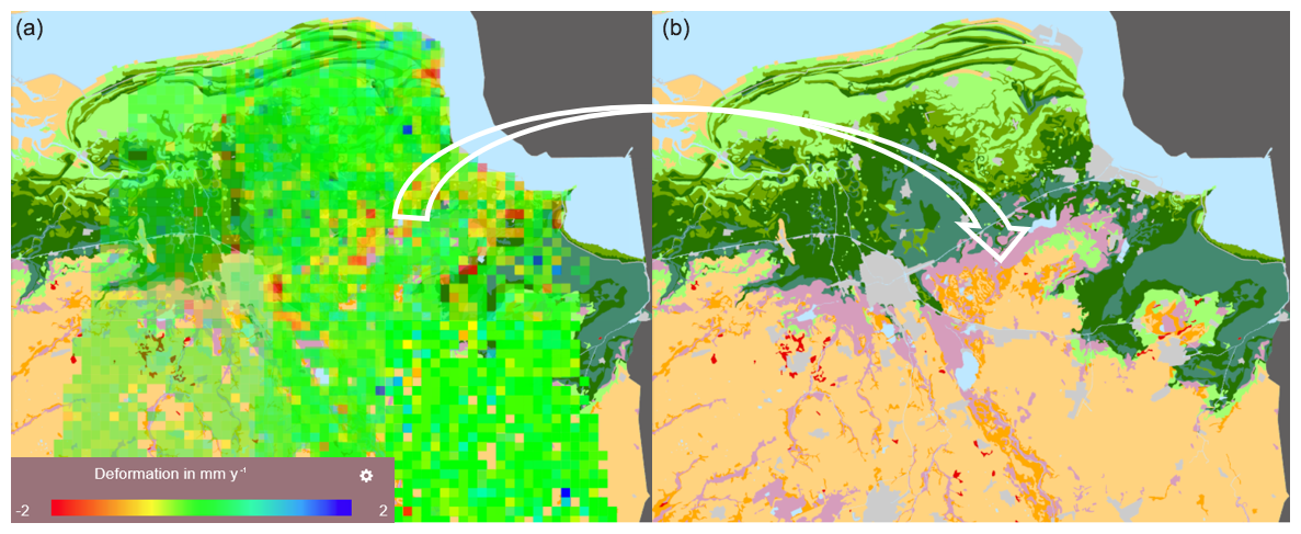
Figure 4Shallow compaction rates (mm yr−1) computed by PS separation based on height above ground level (a), and soil composition (b). The strip with shallow compaction rates of 1–2 mm yr−1 corresponds with the location of peat layers (pink). Source: SkyGeo B.V.
Despite the successful application of InSAR in practice, one of the main concerns is that the quality description of InSAR deformation measurements in terms of precision is not adequate. Often, the error structure is simplified such as neglecting the spatio-temporal correlation between InSAR deformation measurements. The unrealistic quality description could negatively affect decision-making based on the InSAR results.
In order to describe the quality of the InSAR data in terms of precision, it is needed to mathematically describe the spatio-temporal variability of noise components in the data. It should be noted that, in the context of deformation monitoring and modeling, the term noise not only comprises the uncertainty of the measurements itself (scattering and atmospheric noise in InSAR), but it also subsumes all signal (or deformation) components in InSAR observations that are not related to the signal of interest. Therefore, we distinguish two noise components: measurement noise, and idealization noise (level to which the measurements are representative for the signal of interest). Here, the main focus is on the stochastic modeling (covariance matrix) of the InSAR measurement noise (Van Leijen et al., 2020).
In order to evaluate the spatio-temporal variability of the measurement noise, an InSAR dataset over an assumedly signal-free area ( km) in northern Netherlands has been used. A RadarSAT-2 dataset containing 98 radar images acquired between 2009 and 2016 was used for the study. It should be noted that, although the selected area is assumed to be affected minimally by deep and shallow sources, it still could be affected by some residual deformation. In order to isolate the effect of measurement noise, the potential contribution of residual deformation should be subtracted from the data. To do so, for each InSAR point, a linear trend and a periodic annual signal has been estimated and subtracted from the timeseries of InSAR observations. The remaining can be assumed to contain only measurement noise.
From the obtained timeseries of all the points in the selected area, the spatio-temporal empirical variograms are computed using robust algorithms (Cressie and Hawkins, 1980; Genton, 1998) in order to reduce the sensitivity to outliers. The results are visualized in Fig. 5. By visual/qualitative analysis of this figure, we can recognize three different types of behavior: (i) a nugget effect (lower bound of ∼10 mm2), (ii) a spatially correlated signal, and (iii) a temporally correlated signal.
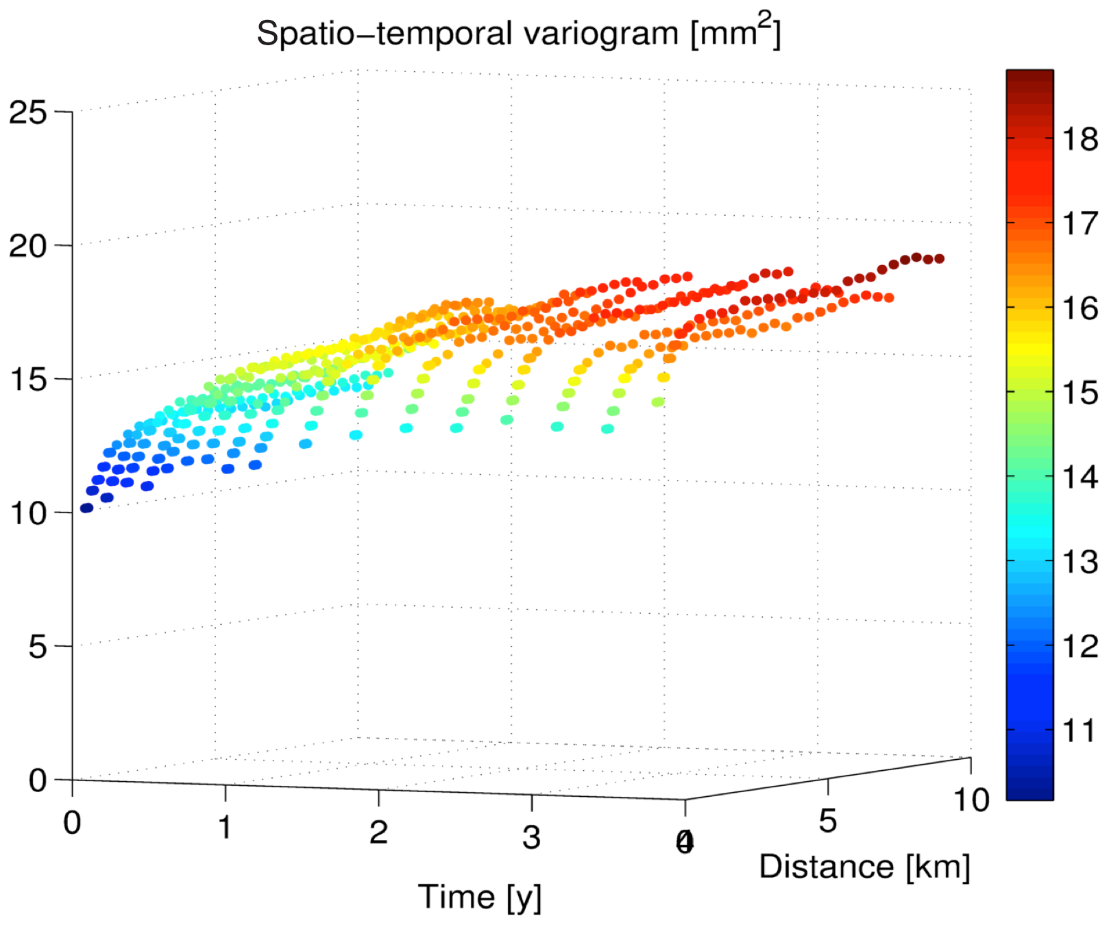
Figure 5Spatio-temporal variograms computed from RadarSAT-2 InSAR data over the assumed stable area.
To combine these three effects in a generic model, the following exponential variogram model has been used:
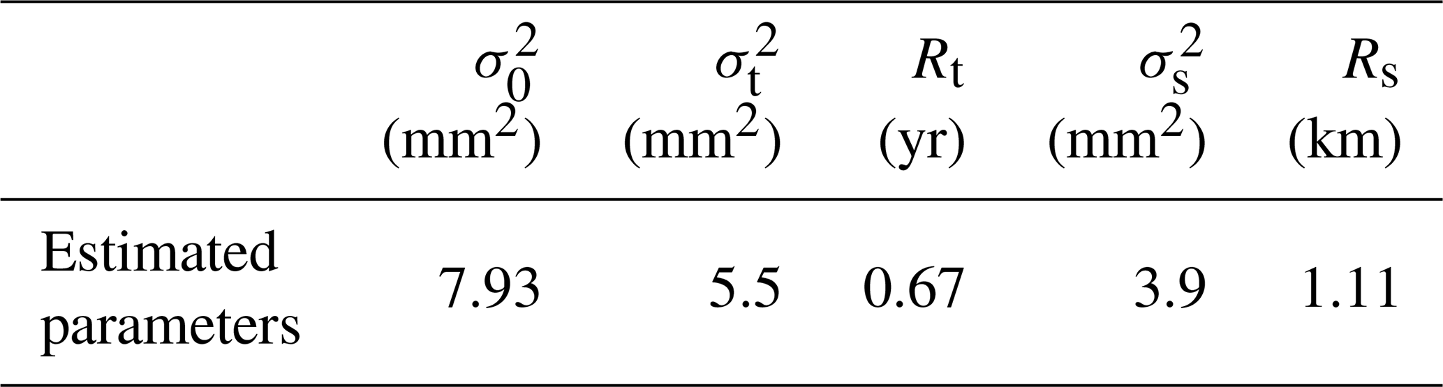
where, Δt and Δd are time difference and spatial distance, γ(Δt,Δd) is the variogram as a function of Δt and Δd , is the variance of the nugget effect, and are the variance of the temporal and the spatial components, and Rt and Rs are the correlation length of the temporal and the spatial components, respectively. The results of the parameter estimation are summarized in Table 1.
Using the estimated variogram model, it is possible to construct the full covariance matrix of measurement noise for the spatio-temporal InSAR data (Yaglom, 1962). Note that the large volume of InSAR data (usually consisting of tens of thousands of points with tens to hundred epochs) result in a huge covariance matrix that is not practically useful due to the computational and numerical limitations. In this regard, a proper data reduction is usually required for InSAR data. Therefore, the covariance matrix of the full dataset should be propagated to the covariance matrix of the reduced dataset. In the context of InSAR processing in Groningen, reduction techniques have been used based on averaging in time and space (e.g. see Samiei-Esfahany and Bähr, 2015). As the averaging-based data reduction can be formulated as a linear operator (e.g., as yreduced=Ayfull), the covariance matrix of the full dataset can be propagated to the reduced covariance matrix using the linear error-propagation as
As an example of the reduced dataset, Fig. 6 shows the reduced InSAR timeseries over Groningen area, with spatial averaging over grids of 5×5 km and temporal averaging over 6 month intervals. Note that, in this example of data reduction, the full dataset of 371 890 point-targets and 98 epochs (i.e., in total 36 445 220 observations), has been reduced to 455 spatial grids and 15 epochs (i.e., in total 6825 observations).
With the proposed approach, a reduced InSAR dataset is delivered to the subsurface community, including its full covariance matrix, incorporating both spatial and temporal correlation of data measurement noise. The covariance matrix can be further used as a quality descriptor of the InSAR data, as well as a proper weight matrix in geomechanical and subsurface modeling.
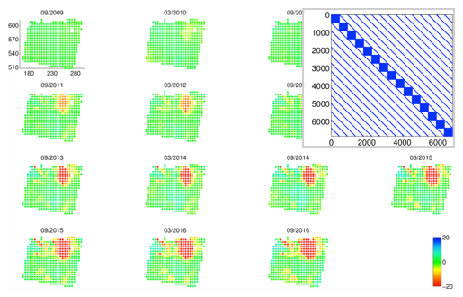
Figure 6Reduced InSAR timeseries over the Groningen area, with spatial averaging over grids of 5×5 km and temporal averaging over 6 month intervals, and the structure of the covariance matrix (upper right). Blue areas show the non-zero elements, which are an indication of both spatial and temporal correlation in the data.
In the NAM GNSS processing methodologies project (Van der Marel, 2020) different methodologies have been investigated with the aim to obtain transparent time series estimates to support conclusions on subsidence rates with realistic confidence levels. The three different processing methodologies that have been investigated are: state-space modeling (SSR), baseline network processing (BSW), and Precise Point Positioning (PPP). An overview of the main characteristics of each method is given in Table 2.
Table 2GNSS processing methodologies. SSR processing has been carried out by 06-GPS using Geo software (Wübbena et al., 2001); BSW by the Dutch Cadastre using the Bernese GNSS software (Dach et al., 2015); PPP by Nevada Geodetic Laboratory (NGL) using Gipsy/Oasis software (Blewitt et al., 2018).
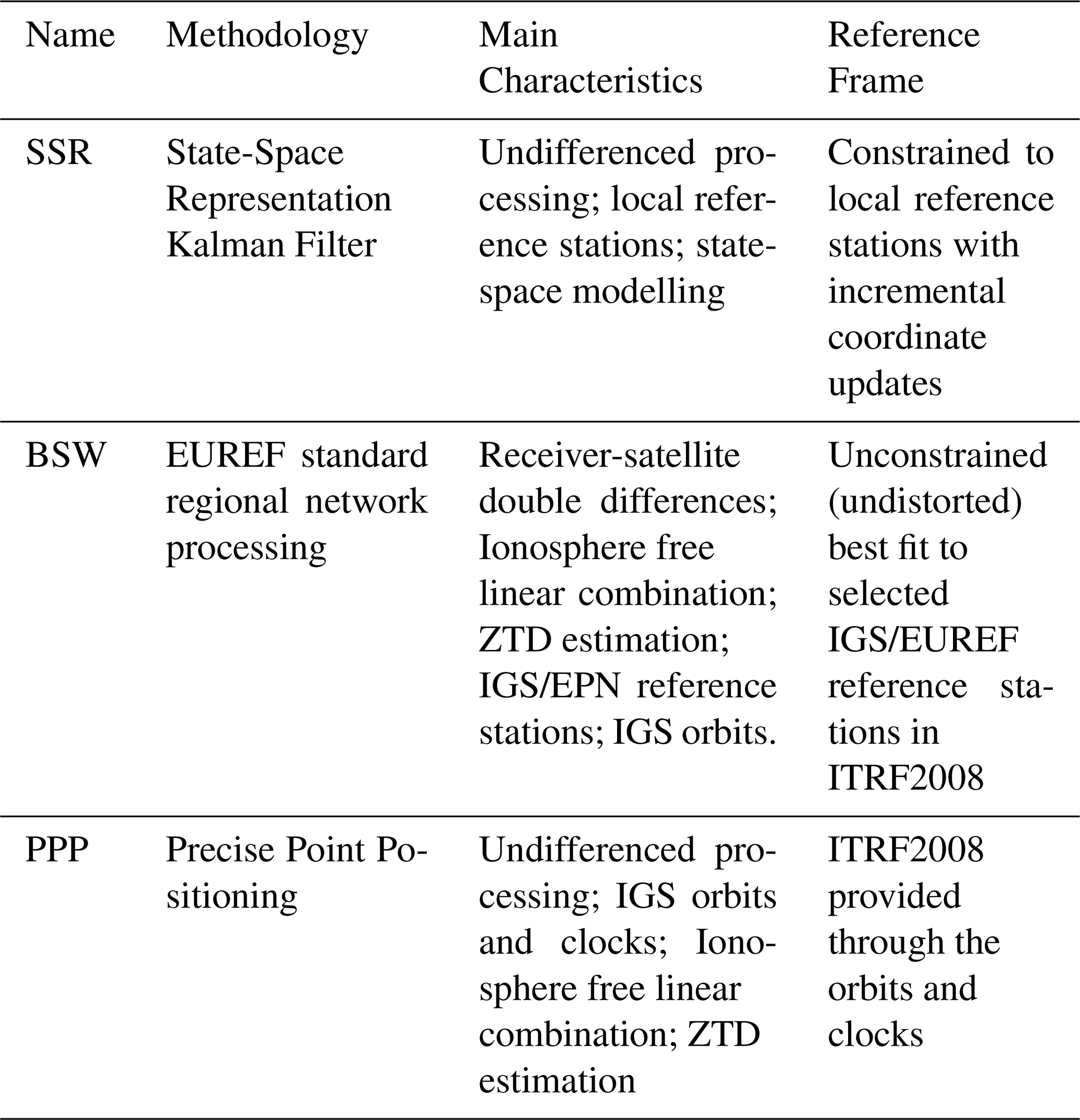
Besides the NAM monitoring and NAM reference stations (of which the coordinates are kept fixed – with incremental updates – in the SSR processing), IGS and EUREF stations have been included in the BSW and PPP processing, as well as the Dutch AGRS and NETPOS stations in the BSW processing.
The time series results have been decomposed into components: a long term trend using a spline function, annual and semi-annual components, temperature influence, atmospheric loading, time series steps (e.g. due to antenna changes), and residuals. In the estimation of the temperature influence and atmospheric loading, temperature and pressure data from the Royal Netherlands Meteorological Institute (KNMI) is used. During a first iteration also two common mode components are estimated, the common mode in the residuals (residual stack), and common mode of the periodic parameters (harmonics, temperature influence, and atmospheric loading). For the estimation of the common mode a subset of the stations is used. The common mode is removed in the second iteration.
All three processing chains estimate, after removal of the common mode, a similar annual, semi-annual, temperature influence and atmospheric loading for each station. The periodic common mode signals themselves are however very different for each solution; the common modes in the BSW and PPP solutions are significantly larger than the common mode in the SSR solutions.
The agreement between the estimated trend signals of the BSW and PPP is good, which is what should be expected because both solutions use ITRF2008 as reference frame. For the final results, the known tectonic motion of the Eurasian plate has been removed in the horizontal component (conversion to ETRS89), but heights stay in ITRF2008. This is because the conversion to ETRS89 introduces a small extra vertical velocity component in the results (∼1 mm yr−1). The cause of this effect lies in the choices that were made for the definition of the transformation between ITRF and ETRS89.
When comparing the BSW and PPP solutions with respect to the SSR solutions, the overall patterns in the time series are similar, however – for some stations – small deviations are present. Figures 7, 8 and 9 show the East, North and Height/Up time series for a selection of Groningen and Wadden Sea GNSS continuous monitoring stations, for the SSR and PPP solution. The BSW solution is similar to the PPP solution, but with a lower noise level.
The reason for the differences lies in the reference stations. The SSR solution is computed in a local reference network. The reference station coordinates are checked periodically by relaxing the coordinate constraints. In case movement is detected in one or more reference stations, the coordinates of the reference stations are updated. For the BSW and PPP, ITRF2008 is used as reference frame. For ITRF2008, reference stations are used that lie well outside the area of interest.
The results indicate that there may be a possibility to further optimize the procedure for the reference stations in the SSR solution. Instead of incremental corrections of a local set of reference station coordinates, the results of the BSW and/or PPP processing could be utilized to strengthen the solution over longer periods. However, a local reference network stays key for high precision local deformation monitoring.
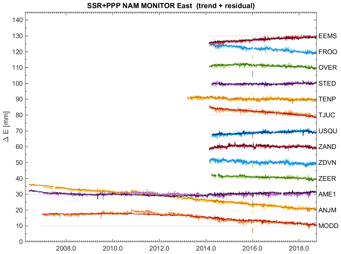
Figure 7GNSS time series East component (relative, mm), PPP (light) and SSR (dark) solution.
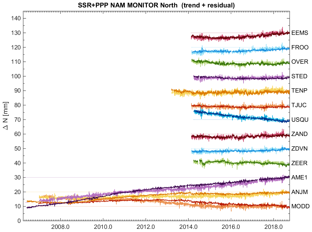
Figure 8GNSS time series North component (relative, mm), PPP (light) and SSR (dark) solution.
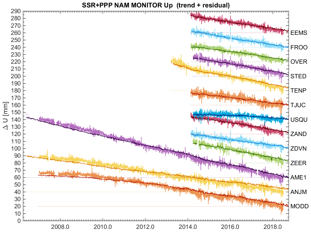
Figure 9GNSS time series Height/Up component (relative, mm), PPP (light) and SSR (dark) solution.
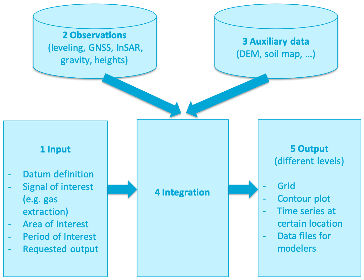
The available observations acquired by the different techniques (levelling, GNSS, InSAR, but potentially also gravity, tilt) are complementary to each other due to their spatial density and coverage, temporal density and coverage, and sensitivity (1D versus 3D). Because of this complementary nature, an integration of the techniques to generate an optimal output product is desirable. However, the differences between the techniques make this integration non-trivial. Conventional geodetic processing methodologies require for instance measurements at common locations (e.g., benchmarks). Therefore, geodetic adjustment and testing procedures are typically applied for each technique/dataset separately, followed by a final integration step.
The Integrated Geodetic Processing (IGP) approach enables the adjustment and testing of the various observation types simultaneously. Hereby, the complementary nature of the techniques is better used. The overall concept of the IGP approach is shown in Fig. 10. The approach meets a number of pre-defined requirements. For instance, the user is able to select the area and period of interest, together with the signal of interest (e.g., surface motion due to deep causes, shallow causes, or the total). Furthermore, various output products can be generated. Before the integration, each dataset is pre-processed to account for certain technique-dependent error sources, such as benchmark identification errors in case of levelling data. Each dataset is accompanied with its covariance matrix. Within the integration step, possible differences between the geodetic datums is accounted for.
Multiple advances have been made in the recent years on monitoring subsidence due to hydrocarbon production in the Netherlands. Integrated Geodetic Reference Stations (IGRS) enable to cross-validate levelling, GNSS and InSAR independent of the deformation cause, and will contribute to minimizing subsurface uncertainties. The application of high-resolution InSAR has quantified shallow deformation components in the Groningen area. The comparison of different GNSS processing methodologies has strengthened the confidence in the information that can be derived from the measurements. The InSAR stochastic model has been improved to incorporate correlated noise structures in an efficient way. All these “ingredients” have consolidated the foundation for integrated geodetic processing for future subsidence monitoring.
Subsidence monitoring data that is publicly available can be accessed via https://www.nlog.nl/geodetische-meetregisters-en-gps-metingen (NLOG, 2020). The geodetic studies described in this paper are covered in the project reports for NAM in the references.
All authors have participated in the collaboration projects between NAM and Delft University of Technology, and contributed to the paper. Particular contributions have been made by SSE on the InSAR stochastic model, by HvdM on GNSS processing methodologies, and by SL on high resolution InSAR in cooperation with SkyGeo B.V.
The authors declare that they have no conflict of interest.
This article is part of the special issue “TISOLS: the Tenth International Symposium On Land Subsidence – living with subsidence”. It is a result of the Tenth International Symposium on Land Subsidence, Delft, the Netherlands, 17–21 May 2021.
The studies described in this paper have been made possible by the contributions from the following parties: high-resolution InSAR processing by SkyGeo B.V.; placement and processing of GNSS receivers by 06-GPS B.V.; GNSS regional network processing by the Dutch Cadastre, and GNSS Precise Point Positioning processing by Nevada Geodetic Laboratory.
Blewitt, G., Hammond, W. C., and Kreemer, C.: Harnessing the GPS data explosion for interdisciplinary science, EOS T. Am. Geophys. Un., 99, https://doi.org/10.1029/2018EO104623, 2018.
Cressie, N. and Hawkins, D. M.: Robust estimation of the variogram: I. Mathematical Geology, 12, 115–125, Springer Berlin Heidelberg, 1980.
Dach, R., Lutz, S., Walser, P., and Fridez, P. (Eds.): Bernese GNSS Software Version 5.2. User manual, Astronomical Institute, University of Bern, 2015.
Genton, M. G.: Highly Robust Variogram Estimation, Mathematical Geology, 30, 213–221, Springer Berlin Heidelberg, 1998.
Hanssen, R.: IPC No. P115850NL00. A radar retroreflector device and a method of preparing a radar retroreflector device, Patent No. 2019103, 2017.
Kamphuis, J. C.: Co-location of geodetic reference points: On the design and performance of an Integrated Geodetic Reference Station, MSc thesis, Delft University of Technology, the Netherlands, 2019.
Nederlandse Aardolie Maatschappij B.V.: Ensemble Based Subsidence application to the Ameland gas field – long term subsidence study part two (LTS-II) continued study, 2017.
NLOG: Geodetische meetregisters en GPS metingen, available at: https://www.nlog.nl/geodetische-meetregisters-en-gps-metingen, last access: 13 March 2020.
Qin, Y., Salzer, J., Maljaars, H., and Leezenberg, P. B.: High resolution InSAR in the Groningen area, project report for NAM, SkyGeo B.V., 2019.
Samiei-Esfahany S. and Bähr, H.: Research and development project for geodetic deformation monitoring, for long-term study on anomalous time-dependent subsidence in the Wadden sea region, Tech. rep., Nederlandse Aardolie Maatschappij B.V., Assen, the Netherlands, 2015.
Van der Marel, H.: Comparison of GNSS Processing Methodologies for Subsidence Monitoring, project report for NAM, Delft University of Technology, 2020.
Van Leijen, F. J., Samiei-Esfahany, S., Van der Marel, H., and Hanssen, R. F.: Improving the Functional and Stochastic Model of InSAR, project report for NAM, Delft University of Technology, 2020.
Wübbena, G., Bagge, A., and Schmitz, M.: RTK networks based on Geo GNSMART – Concepts, Implementation, Results, Proceedings of the National Technical Meeting of the Satellite Division of the Institute of Navigation, ION GPS/2001, September 2001, Salt Lake, USA, 368–378, 2001.
Yaglom, A. M.: An Introduction to the Theory of Stationary Random Functions, Series of selected Russian publications in the mathematical sciences, Prentice-Hall, 1962 (revised English edition translated and edited by Richard A. Silverman, Dover Publications, Mineola, New York, 2004).