Changes in soil erosion and sediment transport based on the RUSLE model in Zhifanggou watershed, China

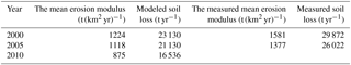
In this paper, changes of sediment yield and sediment transport were assessed using the Revised Universal Soil Loss Equation (RUSLE) and Geographical Information Systems (GIS). This model was based on the integrated use of precipitation data, Landsat images in 2000, 2005 and 2010, terrain parameters (slope gradient and slope length) and soil composition in Zhifanggou watershed, Gansu Province, Northwestern China. The obtained results were basically consistent with the measured values. The results showed that the mean modulus of soil erosion is 1224, 1118 and 875 t km⁻² yr⁻¹ and annual soil loss is 23 130, 21 130 and 16 536 in 2000, 2005 and 2010 respectively. The measured mean erosion modulus were 1581 and 1377 t km⁻² yr⁻¹, and the measured annual soil loss were 29 872 and 26 022 t in 2000 and 2005. From 2000 to 2010, the amount of soil erosion was reduced yearly. Very low erosion and low erosion dominated the soil loss status in the three periods, and moderate erosion followed. The zones classified as very low erosion were increasing, whereas the zones with low or moderate erosion were decreasing. In 2010, no zones were classified as high or very high soil erosion.

1 Introduction

Soil erosion is a process which refers to the destruction, separation, removal and sedimentation of the earth's surface soil and its parent material caused by hydraulic, wind, freezing and thawing, gravity and other external forces (Meyer, 1984). Soil erosion has caused a set of ecological and environmental problems such as land degradation, soil fertility loss, river siltation, making it a global research focus. Since the 1950s, to quantify soil loss and determine its risk, a number of soil erosion models were established based on measured data or the results of previous studies, and numerous research results were obtained using Geographical Information Systems (GIS) and remote sensing (RS). One of the most applied models to estimate soil erosion is the Universal Soil Loss Equation (USLE) and its modified version the Revised Universal Soil Loss Equation (RUSLE). Lu et al. (2001) used GIS and the RUSLE model to map and quantitatively predict patch and gully erosion in Australia. Liu (2002) established China's Soil Erosion Prediction Equation (CSLE) by the study of a slope erosion prediction model. Gao et al. (2015) calculated the soil erosion modulus in the Loess Plateau of China in 2010 by using the RUSLE model. Because of the complex landscape, the soil erosion status varies in the Loess Plateau. This paper focused on analysing the land use pattern, vegetation distribution and soil erosion status based on the RUSLE model and the impact of slope changes and land use types on erosion by using RS and GIS in the Zhifanggou watershed, Loess Plateau. The aim was to analyse the evolution of soil erosion in a complete and systematic way and provide a reference basis for soil and water loss prevention in hilly and gully regions of the Loess Plateau.

Figure 1 The topography of Zhifanggou watershed.

2 Materials and methods

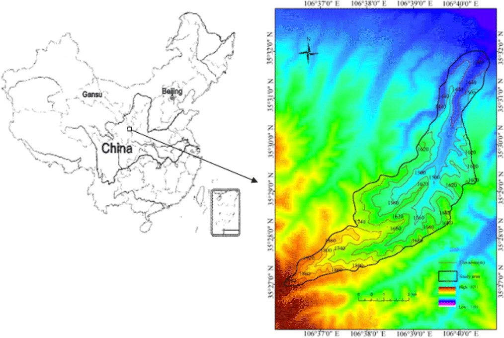
2.1 Study area

Zhifanggou watershed is located in the gully area of Longdong Loess Plateau, Gansu Province, Northwestern China. This watershed has been a key management and experimental area in the Yellow River Basin since 1954. Many management approaches have been carried out to reduce soil erosion, such as soil and water conservation measures, renovating barren slopes and terraces. Ten hydrology and rainfall observation stations were set up to observe rainfall, evaporation, runoff, flood and sediments for more than 50 years.

Figure 1 presents the Zhifanggou watershed. It is one of the tributaries to the Jinghe river and is located south of Pingliang City, China. The area of Zhifanggou watershed is 18.98 km². It extends between the latitudes of 35^∘26^′ and 35^∘33^′ N and longitudes of 106^∘37^′ and 106^∘42^′ E. The watershed altitude ranges from 1365 to 2104 m. The main channel length is 15.77 km and the mean channel slope is 4.34 %.

2.2 RUSLE model

The factors in the RUSLE model include rainfall erosivity, soil erodibility, slope length and steepness, vegetation cover and management, and supporting practices (Wischmeier and Smith, 1965). In order to estimate the soil loss, meteorological data, soil information, RS data and a digital elevation model (DEM) were used as detailed below.

1. Three Landsat Thematic Mapper images of the study area from May 2000, May 2005 and July 2010, with 30 m of spatial resolution were used.

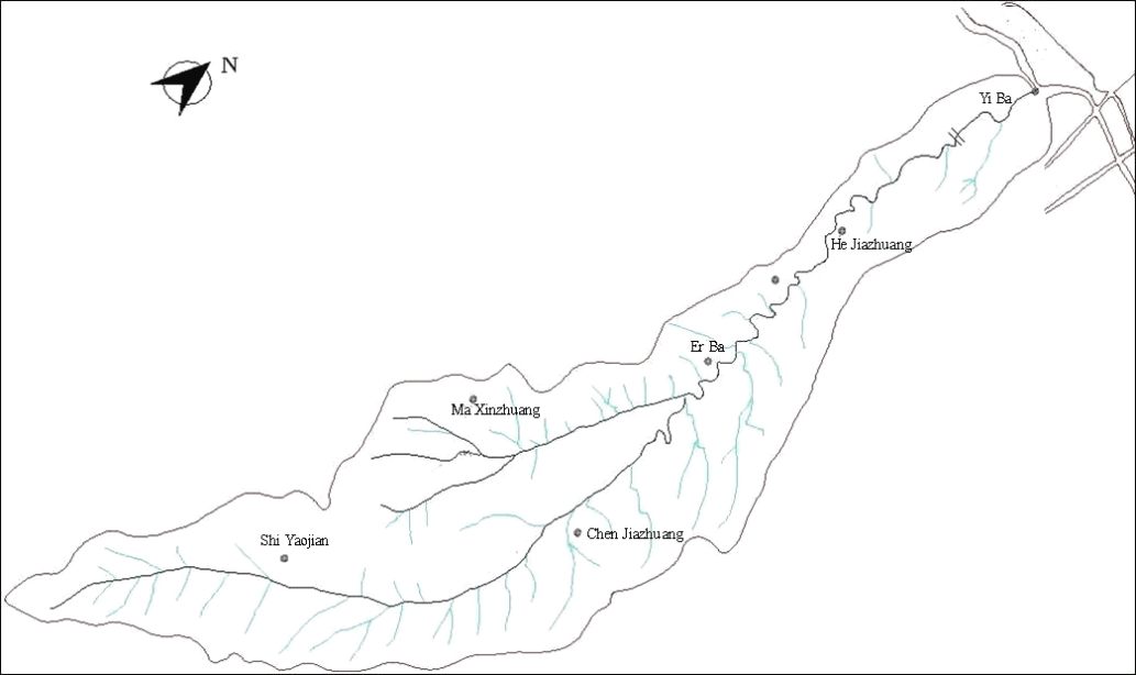
2. Daily rainfall data from 1981 to 2004 were obtained from the first and second dams and Hejiazhuang hydrological stations, and Majiaxinzhuang, Chenjiazhuang and Shiyaojian precipitation stations. Because of the lack of observers and funds, the observations were withdrawn in 2005 and merged into one station, named Pingliang hydrological station. Therefore annual rainfall data of Pingliang hydrological station were used from 2005 to 2010.

3. A DEM of 30 m spatial resolution was obtained.

4. Soil information (including organic matter content and texture) for the study area was obtained from the analysis of soil samples.

Figure 2 The distribution of rainfall and hydrologic stations.

Figure 3 The spatial distribution of rainfall erosivity factor.

Figure 4 The spatial distribution of soil samples.

The RUSLE model is used to estimate soil loss by water-caused erosion (Renard et al., 1997; Duarte et al., 2016). The mathematical expression of RUSLE is

$$\begin{array}{}\text{(1)}& A=R\times K\times LS\times C\times P\end{array}$$

where A is the mean annual soil loss (t km⁻² yr⁻¹), caused by rainfall and runoff. R is the rainfall erosivity factor (MJ mm hm⁻² h⁻¹), which reflects the potential soil erosion caused by rainfall. In RUSLE, it is defined as the product of rainfall energy and maximum rainfall intensity of 30 min. K is the soil erodibility factor (t h MJ⁻¹ mm⁻¹), which represents

the amount of soil erosion caused by unit rainfall force in the standard plot. It is used to reflect soil sensitivity to erosion. The slope length and steepness (LS) factor represents the effect of topography on soil erosion, L is the slope length factor and defined as a power function of slope length. S is the slope steepness factor. The vegetation cover factor (C) represents the ratio of soil loss from an area with specified cover and management to soil loss from an identical area in continuous fallow. The conservation support practice factor (P) refers to the ratio of amount of soil loss when soil and water conservation measures, such as contouring or terracing, have been implemented to the original soil loss from sloping land. (Renard et al., 1991; Renard and Ferreira, 1993; Farhan and Nawaiseh, 2015). Soil losses estimated from RUSLE were compared with the measured values which were calculated using the measured annual runoff and suspended sediment of Zhifanggou watershed.

2.2.1 Rainfall erosivity factor (R)

The R factor reflects the potential soil erosion caused by rainfall. In this paper, R was calculated from the original algorithm of

the USLE model proposed by Wischmeier and Smith (1978). The equation is:

$$\begin{array}{}\text{(2)}& R=\sum E\cdot I_{\mathrm{30}}R=\sum E\cdot I_{\mathrm{30}}\end{array}$$

where E is the kinetic energy in a single rainfall event (MJ hm⁻²). It may be counted as a single event if the rainfall is intermittent within 2 h, otherwise the rainfall will be treated twice; I₃₀ is the maximum rainfall intensity in 30 min (mm h⁻¹).

The equation used to calculate E is:

$$\begin{array}{}\text{(3)}& {\displaystyle }& {\displaystyle }{m}_{\text{e}}=\left\{\begin{array}{l}\mathrm{0.119}+\mathrm{0.0873}lg\left(m_{\text{i}}\right),m_{\text{i}}\le \mathrm{76}\\ \mathrm{0.283},m_{\text{i}}>\mathrm{76}\end{array}\right.\text{(4)}& {\displaystyle }& {\displaystyle }E=\sum m_{\text{e}}\cdot P_{m}E=\sum m_{\text{e}}\cdot P_m\end{array}$$

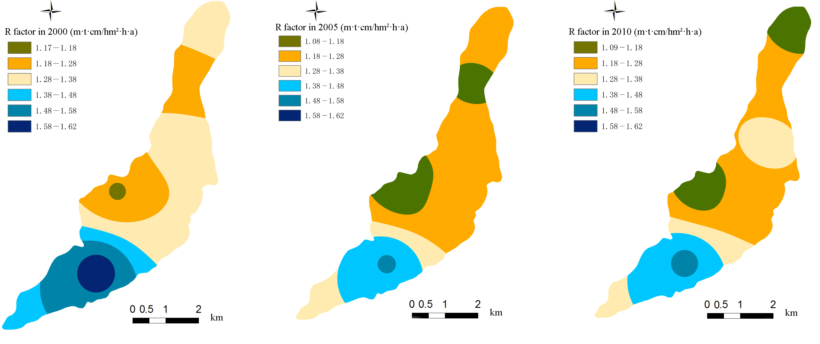
Where m_e is the unit kinetic energy during one rainfall event (MJ mm⁻¹ hm⁻²); m_i is the rainfall intensity corresponding to a certain period (mm h⁻¹); P_m is the total rainfall corresponding to a certain period (mm). Based on the interpolation and extension of rainfall data, mean annual rainfaIl erosivity of six stations were calculated during three periods: before 2000, 2001 to 2005 and 2006 to 2010. The distribution of the six stations is shown in Fig. 2. The rainfall erosivity map (Fig. 3) was obtained by the inverse distance weighting method (IDW) which has been shown to be most suitable for rainfall interpolation in this area of China (Bai et al., 2012).

2.2.2 Soil erodibility factor (K)

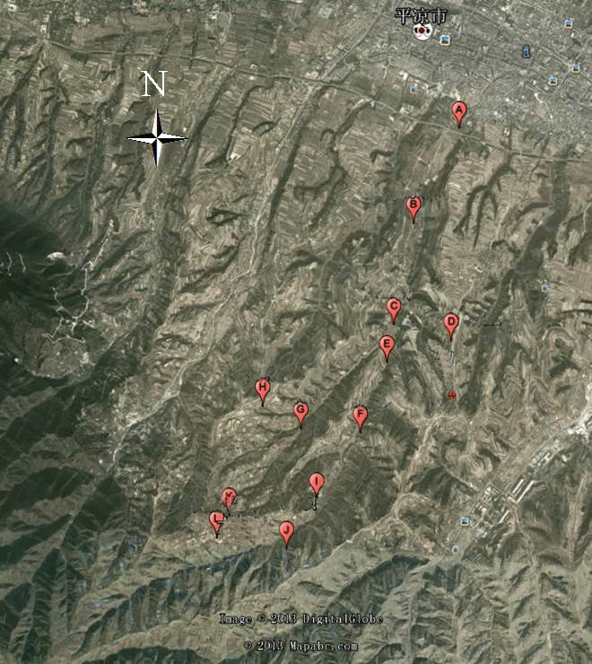
According to the equation, the greater the K value, the greater the risk of soil erosion and vice versa. Twelve soil samples were collected in this watershed and analyzed to determine particle size (sand, silt, clay) and organic matter content in order to calculate K. The distribution of the 12 soil samples is shown in Fig. 4.

There are many methods to calculate the K factor (Wischmeier and Smith, 1978). Considering that the parameters of the EPIC method are measured readily and the method is relatively mature, K was calculated by using the EPIC (erosion-productivity impact calculator) model (Sharpley and Williams, 1990):

$$\begin{array}{}\text{(5)}& {\displaystyle }\begin{array}{l}K=\left\{\mathrm{0.2}+\mathrm{0.3}\exp \left[-\mathrm{0.0256}\text{SAN}\left(\mathrm{1.0}-\text{SIL}/\mathrm{100}\right)\right]\right\}{\left({\displaystyle \frac{\text{SIL}}{\text{CLA}+\text{SIL}}}\right)}^{\mathrm{0.3}}\\ -\left(\mathrm{1.0}-{\displaystyle \frac{\mathrm{0.25}C}{C+\exp \left(\mathrm{3.72}-\mathrm{2.95}\right)}}\right)\left(\mathrm{1.0}-{\displaystyle \frac{\mathrm{0.7}\mathrm{SN}\mathrm{1}}{\mathrm{SN}\mathrm{1}+\exp \left(-\mathrm{5.51}+\mathrm{22.9}\mathrm{SN}\mathrm{1}\right)}}\right)\end{array}\end{array}$$

where SAN, SIL, CLA and C are sand, silt, clay and organic carbon (%).

Figure 5 Soil erodibility map (K).

Figure 6 Spatial distribution of the slope steepness factor.

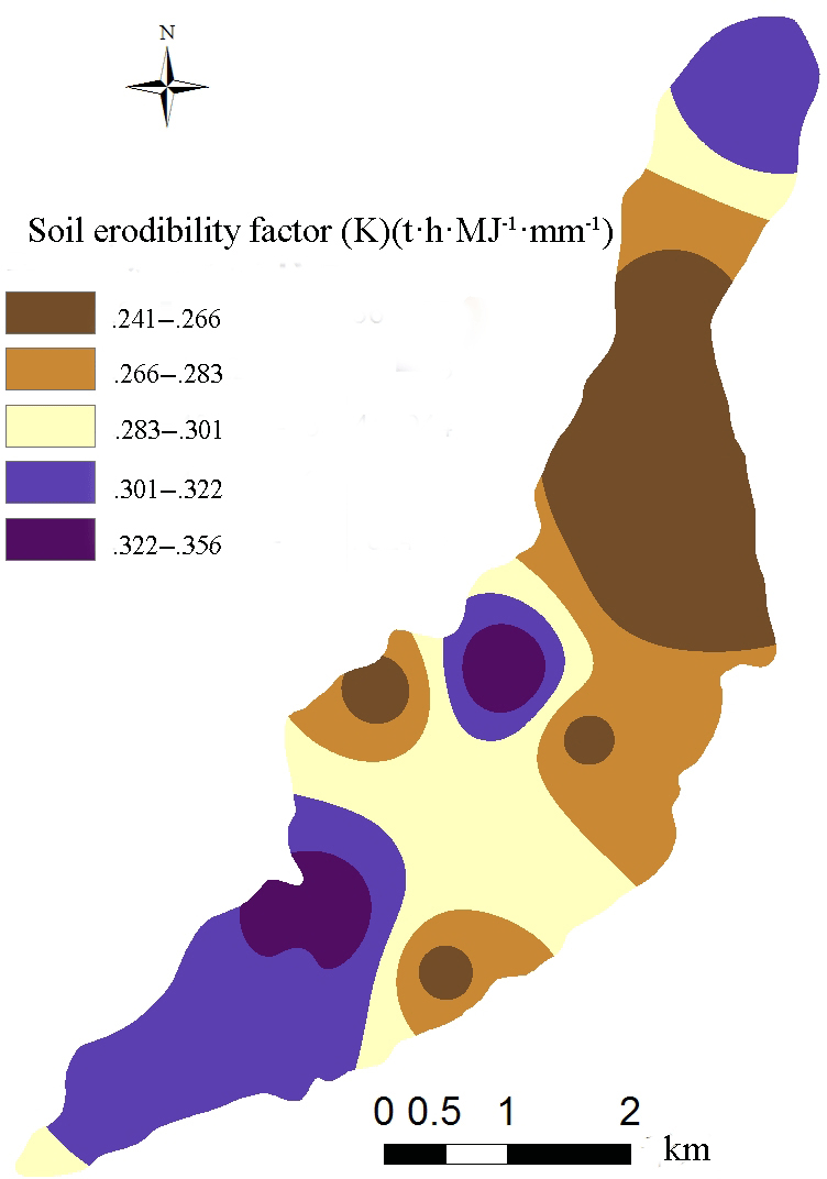
The equation used to calculate SN1 is:

$$\begin{array}{}\text{(6)}& {\displaystyle }\text{SN1}=\mathrm{1}-\text{SAN}/\mathrm{100}.\end{array}$$

The K factor map (Fig. 5) was obtained by the kriging spatial interpolation method which is more suitable for soil moisture spatial interpolation in the Loess Plateau region (Yao et al., 2013).

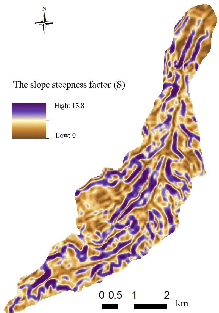
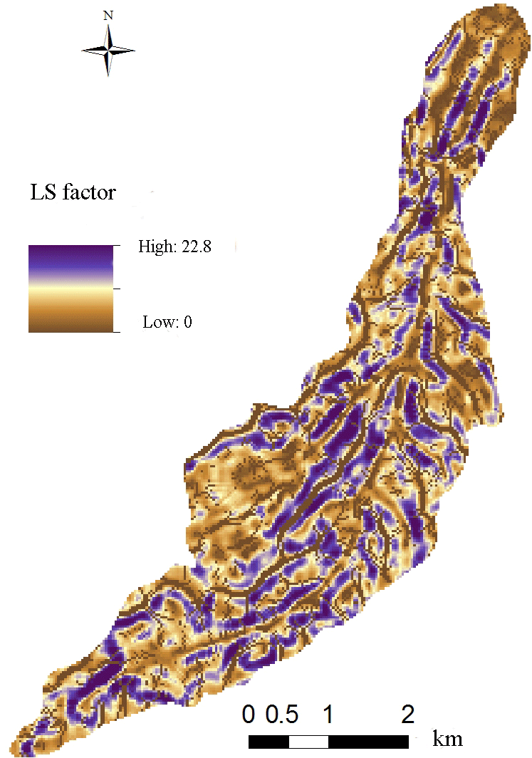
2.2.3 Topographic factor (LS)

The slope steepness factor (S) reflects the influence of slope gradient on erosion (Lu et al., 2001). The greater the mean slope, the greater the potential risk of soil separation and the more severe the soil erosion. S is calculated by using the equations established by Liu et al. (1994) and Liu (2002) as follows:

$$\begin{array}{}\text{(7)}& \left\{\begin{array}{ll}S=\mathrm{10.80}\times \sin \mathit{\theta }+\mathrm{0.03}& \mathit{\theta }<{\mathrm{5}}^{\circ }\\ S=\mathrm{16.80}\times \sin \mathit{\theta }-\mathrm{0.50}& {\mathrm{5}}^{\circ }\le \mathit{\theta }<{\mathrm{10}}^{\circ }\\ S=\mathrm{21.91}\times \sin \mathit{\theta }-\mathrm{0.96}& \mathit{\theta }\ge {\mathrm{10}}^{\circ }\end{array}\right.\end{array}$$

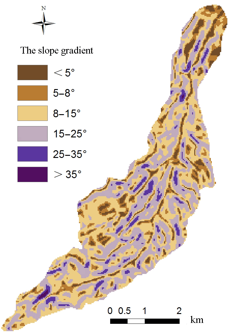
The DEM data of the basin were used to obtain the gradient grid by using the Surface Analysis function in the Spatial Analyst module of ArcGIS.

The slope data were divided into categories of < 5, 5–8, 8–15, 15–25, 25–35, ≥ 35^∘ by using the Reclassify option in 3D Analyst module of ArcGIS. The spatial distribution of slope gradient is shown in Fig. 7.

Figure 7 Spatial distribution of slope steepness.

Figure 8 Spatial distribution of slope length.

Figure 9 Spatial distribution of L factor values.

Figure 10 Spatial distribution of LS factor values.

Figure 11 The spatial distribution of vegetation cover factor in the three study years.

Figure 12 The spatial distribution of land use patterns in the three study years.

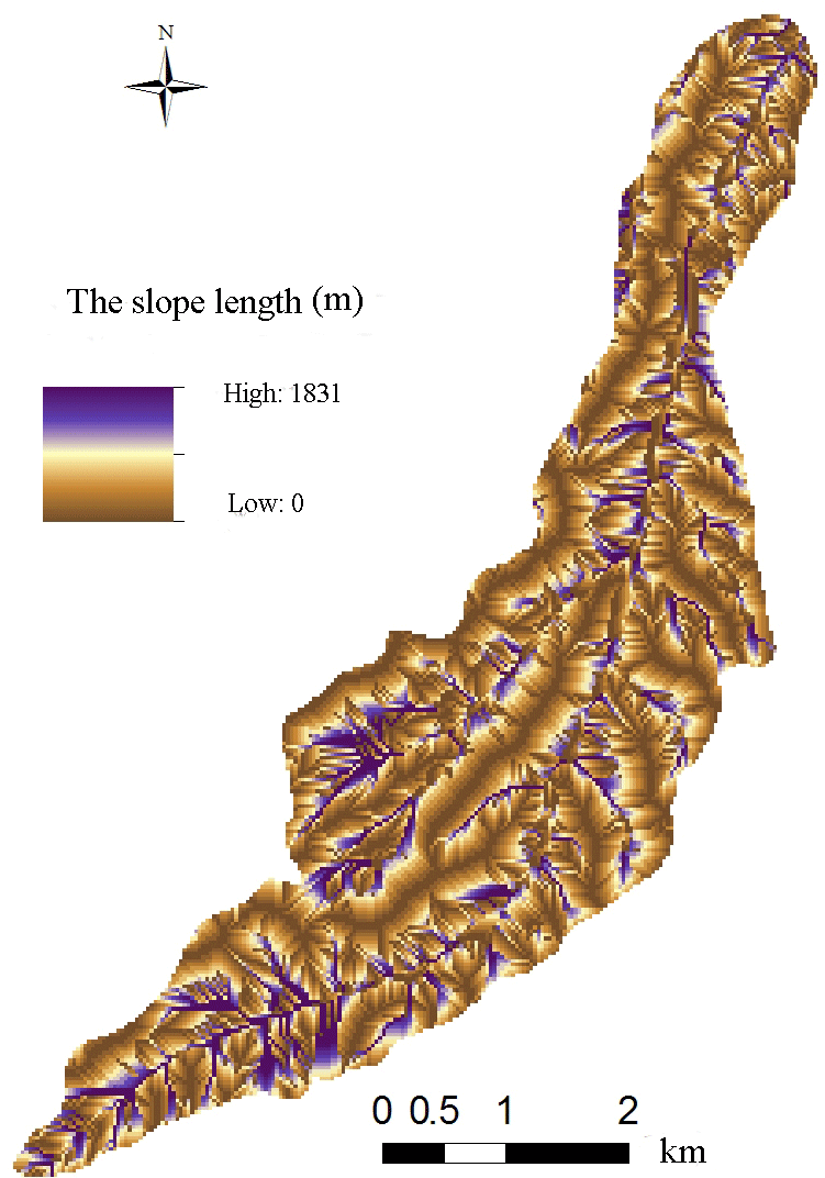
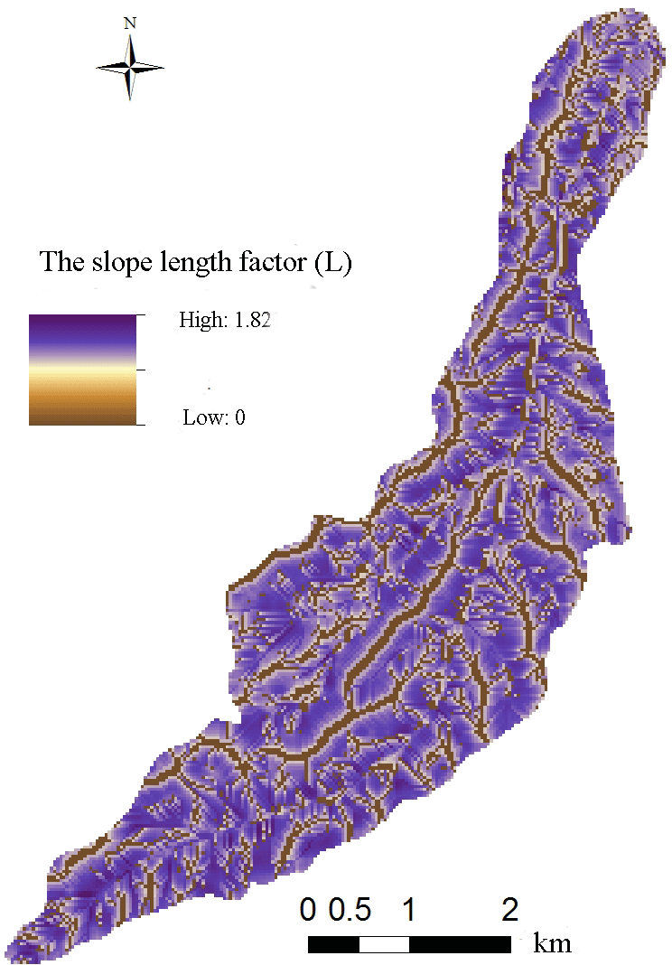
The slope length factor (L) represents the effect of slope length on erosion. The longer the slope length, the greater the flow, and the more severe the soil erosion. L was calculated by the classical method of USLE, as follows:

$$\begin{array}{}\text{(8)}& {\displaystyle }& {\displaystyle }L={\left(\mathit{\lambda }/\mathrm{22.13}\right)}^{\mathit{\alpha }}\text{(9)}& {\displaystyle }& {\displaystyle }\mathit{\alpha }=\mathit{\beta }/\left(\mathit{\beta }+\mathrm{1}\right)\text{(10)}& {\displaystyle }& {\displaystyle }\mathit{\beta }=\left(\sin \mathit{\theta }/\mathrm{0.0896}\right)/\left|\mathrm{3.0}\left(\sin {\mathit{\theta }}^{\mathrm{0.8}}+\mathrm{0.56}\right)\right|\end{array}$$

Where λ is the slope length (m), 22.13 represents the slope length of the standard district (m), α is the slope length exponent, β indicates the ratio of rill to interrill erosion and θ represents the slope gradient extracted from the DEM data. The DEM was used to obtain the slope length (Fig. 8) by using ArcGIS.

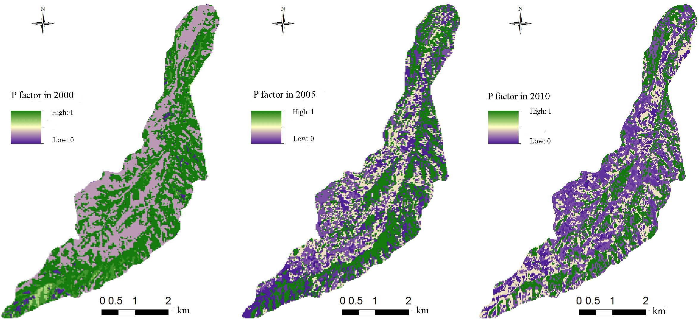
Figure 13 The spatial distribution of the conservation support practice factor in the three study years.

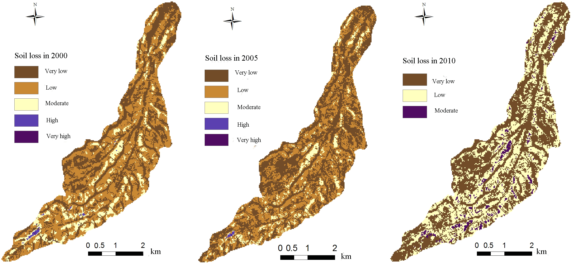
Figure 14 The spatial distribution of soil loss estimated using RUSLE for each of the study years.

Considering there is no function to calculate the slope length directly in ArcGIS, we first calculated the flow direction of the grid by the surface runoff simulation. Then we calculated the flow accumulation of the grid. Based on the extraction of the zero value of the flow accumulation, the ridge line was obtained. Finally, the slope length was calculated using the generated ridge line.

Based on the Map algebra function of ArcGIS, L was calculated according to the equation and is shown in Fig. 9. Multiplying the spatial distribution of the S and L factors, the LS value distribution is obtained, as shown in Fig. 10.

Table 1 Conservation support practice factor (P) value.

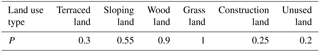
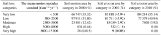
Table 2 Areas of different categories of soil loss in the study catchment (ha).

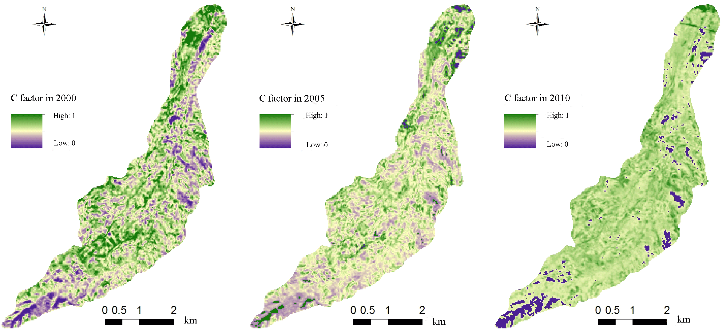
2.2.4 Vegetation cover factor (C)

The vegetation can effectively protect the surface soil from direct impact by rainfall and play an important role in moderating surface runoff, extending moisture penetration time and enhancing soil impact resistance. The Normalized Difference Vegetation Index (NDVI) reflects the vegetation coverage well. The NDVI data used in this paper (May 2000, May 2005 and July 2010) was collected from the International Scientific Data Service Platform. The vegetation cover is calculated by the classical method (Tan et al., 2005), as follows:

$$\begin{array}{}\text{(11)}& \mathrm{\text{fg}}=(\text{NDVI}-{\text{NDVI}}_{min})/({\text{NDVI}}_{max}-{\text{NDVI}}_{min})\times \mathrm{100}\end{array}$$

where fg is the vegetation coverage (%), NDVI_max and NDVI_min are the maximum and minimum values of NDVI. By using the method of Cai et al. (2000), C is calculated as follows (in order to prevent a negative C value, the method is slightly modified as below). The spatial distribution of C was calculated for each of the study years 2000, 2005 and 2010 and is shown in Fig. 11.

$$\begin{array}{}\text{(12)}& C=\left\{\begin{array}{ll}\mathrm{1}& \mathrm{0}\le \text{fg}<\mathrm{0.095}\\ \mathrm{0.6508}-\mathrm{0.3436}{\text{log}}_{\mathrm{10}}\left(\text{fg}\right)& \mathrm{0.095}\le \text{fg}\le \mathrm{78.3}\\ \mathrm{0}& \text{fg}>\mathrm{78.3}\end{array}\right.\end{array}$$

2.2.5 Conservation support practice factor (P)

The value of P ranges from 0 to 1, where 0 indicates good conservation practice and 1 indicates poor conservation practice (Wischmeier and Smith, 1978). The P value was assigned according to Liu et al. (2001), Liu (2006) and Zhao et al. (2016).

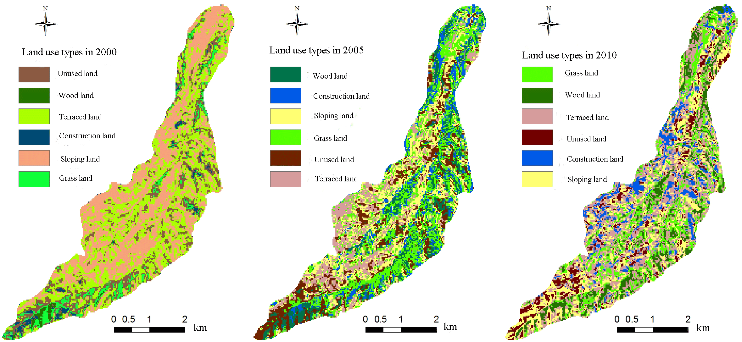
RS images in 2000, 2005 and 2010 were classified and re-processed in ENVI4.8 (Pan et al., 2013) to obtain land use patterns, as shown in Fig. 12. The land use is divided into six categories: terraced land, sloping land, wood land, grass land, construction land and unused land, as shown in Table 1. The P factor was assigned according to field investigation and agricultural practices observed in the study basin. The P values of terraced land and construction land were close to 0 due to good soil and water conservation measures. The P values of wood land and grassland were 1, due to the scattered distribution of these land uses and lack of artificial protection measures. The results are assigned to the RS image classification map to obtain raster maps of P for each of the study years, as shown in Fig. 13.

2.2.6 Soil erosion map

The spatial distribution of soil loss in 2000, 2005 and 2010 were obtained from multiplication of the five factors (R, K, LS, C and P) using the grid calculator of Spatial Analystin ArcGIS software.The spatial distribution of the soil loss was obtained and presented in Fig. 14. Table 2 shows the modeled soil loss areas calculated across all grid squares in the basin for each study year according to the classification standards for soil erosion of China in 2007. The total modeled soil erosion amount was calculated as the sum of the modeled soil losses in all grid squares. The mean modelled erosion modulus was calculated by dividing the total soil erosion amount by the total area of the basin. The modeled and measured erosion modulus are shown in Table 3. Because of the lack of observers and funds, soil erosion was not measured in the study area in 2010, so there is no measured value for 2010 in Table 3.

Table 3 Comparison of modeled and measured annual soil loss across the whole study catchment.

3 Results and discussion

3.1 Estimation of soil erosion

According to Fig. 14 and Table 3, the estimates of soil loss made using RUSLE were basically consistent with the measured values. Soil erosion in the study area is mainly classified as very low and low. In 2000, 2005 and 2010, very low erosion accounted for 35.32, 45.94 and 55.14 % of the total catchment area, low erosion area accounted for 51.80, 45.92 and 40.94 %, and moderate erosion accounted for 12.42, 7.97, 3.92 %. The areas classified as very low erosion are increasing, whilst the areas with low or moderate erosion are decreasing. It can be concluded therefore that the erosion intensity is decreasing. In 2010, no areas were classified as high or very high soil erosion. A similar trend was reported by Gao et al. (2015) of increasing areas of very low erosion in the Loess Plateau from 2010. The parameters in the model can significantly impact the accuracy of the result, so the lack of quantitative description of the P values (conservation support practice factor) may decrease the accuracy of the results. More accurate characterization of P values is an important area for future study.

3.2 Characteristics of soil erosion under different land use patterns

Land use has changed the micro-terrain and original vegetation types and their coverage in the Zhifanggou watershed, affecting the dynamics of soil erosion and resistance. Using the Spatial analysis function of ArcGIS, the land use pattern map and the modelled soil loss map in 2010 were superimposed in order to assess the soil erosion characteristics of the different land use types.

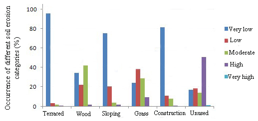
Figure 15 Characteristics of soil erosion under different land use patterns across all three study years.

Figure 15 shows the intensity of soil erosion is different among different land use types. The soil erosion intensity of terraced fields, sloping land and construction land is mainly very low due to soil and water conservation measures. The erosion intensity of wood land is mainly moderate, and the grassland is mainly low. Because the distribution of wood land is intermixed with natural grassland, and also due to the lack of artificial soil protection measures, the erosion intensity is high. The erosion intensity of unused land is very high, because its surface vegetation is sparse and the land is difficult to manage.

These results are consistent with the findings of Zhang (2016) that the construction of terraced fields reduced the area of mild erosion intensity in the basin and increased the area of low erosion intensity, which had a positive effect on soil and water conservation.

3.3 Characteristics of soil erosion under different slope gradients

Using the Spatial analysis function of ArcGIS, the slope gradient map and the soil loss map in 2010 were superimposed in order to examine soil erosion intensity under different slope gradients.

Figure 16 shows that the intensity of soil erosion is different among different land slope gradients. The soil erosion intensity of slopes < 5^∘ is mainly very low. Areas of very low erosion decreased and low and moderate erosion increased in the 5–15^∘ slope categories. Areas of very low and low erosion decreased and moderate erosion increased in the 15–35^∘ slope categories. On slopes greater than 35^∘, there is some high soil erosion and the moderate erosion area increases. In conclusion, in the same conditions, estimated soil erosion increased obviously with the increase of slope in the range of 0–15^∘. When the slope is greater than 15^∘, soil erosion intensity increased only slightly with the increase of slope. These results are consistent with the findings of Abdo and Salloum (2017) that soil erosion rates increased with increasing slope and peaked on steep slopes primarily.

4 Conclusions

From 2000 to 2010, the amount of soil erosion was reduced yearly, and the main erosion status in the three periods was very low and low erosion. During the study period, the areas classified as very low erosion were increasing, whilst the areas with low or moderate erosion decreased. Thus erosion intensity decreased over time across the study watershed, with areas of high and very high erosion disappearing by 2010. The soil erosion intensity of terraced fields, sloping land and construction land were mainly very low due to soil and water conservation measures. The erosion intensity of wood land was mainly moderate, and the grassland was mainly low. Soil erosion increases with increasing slope in the range of 0–15^∘. When the slope is greater than 15^∘, the change of slope has little effect on the distribution of soil erosion intensity.

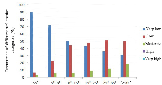
Figure 16 Characteristics of soil erosion under different slope gradient across all three study years.

The estimates of soil loss using RUSLE are basically consistent with the measured values. Hence the RUSLE model can be used to assess soil erosion conditions in the Zhifanggou watershed and help to target areas in the watershed for maintenance and management procedures to reduce soil erosion risk. A follow-up study should analyse the sensitivity of the model parameters and simplify the parameter requirements of the soil erosion model to effectively simulate soil erosion.