Land subsidence modelling using a long short-term memory algorithm based on time-series datasets

With the rapid growth of data volume and the development of artificial intelligence technology, deep-learning methods are a new way to model land subsidence. We utilized a long short-term memory (LSTM) model, a deep-learning-based time-series processing method to model the land subsidence under multiple influencing factors. Land subsidence has non-linear and time dependency characteristics, which the LSTM model takes into account. This paper modelled the time variation in land subsidence for 38 months from 2011 to 2015. The input variables included the change in land subsidence detected by InSAR technology, the change in confined groundwater level, the thickness of the compressible layer and the permeability coefficient. The results show that the LSTM model performed well in areas where the subsidence is slight but poorly in places with severe subsidence.

1 Introduction

The continuous over-pumping of groundwater can result in dramatic drawdown and regional land subsidence, threatening the living environment. Land subsidence is often related to anthropogenic factors that can cause economic losses and casualties, such as municipal infrastructure damage, cracks in transport facilities, and building fractures.

Land subsidence is a complex process influenced by the interaction of anthropogenic activities and the hydrogeological environment. It often develops unevenly and seasonally and can display hysteresis depending on the soil mechanical properties (Ezquerro et al., 2014; Miller and Shirzaei, 2015; Bonì et al., 2016; Gao et al., 2018; Haghighi and Motagh, 2019).

Previous studies on the mechanism of land subsidence were based on the well-understood constitutive model, and the numerical simulation model was established to simulate the future displacement. However, explicit description of hydrogeological information which may have space–time sparseness is required to do so accurately. This constrains its application for large areas. The grey model (GM) based on grey theory is an alternative model to predict the short-term land subsidence, but it ignores the non-linear characteristic of land subsidence. Some researchers proposed the modified GM model combined with artificial neural network (ANN) or other algorithms to deal with the non-linear features (Li et al., 2007). These methods can have a good short-term prediction and perform well when data volume is small, while the deep information cannot be mined when the data volume is large and cannot be used in long-term prediction.

The long short-term memory (LSTM) model is a deep-learning method that can process a large volume of time-series data and forecast the value of the next moment. It constructs a multilayer neural network to excavate the temporal dynamic features of historical data, considering the non-linearity and temporal dependency characteristics. The prediction period depends on the time interval of the input data. It has been successfully applied to PM_2.5 concentration forecasting, which is a temporal–spatial phenomenon (Qi et al., 2019), but no research used this method to simulate the land subsidence.

With the rapid growth of land subsidence data volume obtained by InSAR technology, the application of deep-learning methods of recent studies shows its potential in time-series land subsidence modelling (Yu et al., 2018). In this paper, we utilized the LSTM method to model the land subsidence under multiple influencing factors.

2 Study area and datasets

2.1 Study area

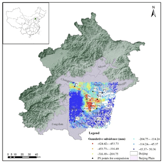
The study area is located in the Beijing Plain, where the largest cumulative land subsidence from 2011 to 2015 had been reached at 624.42 mm, as shown in Fig. 1. Due to urban sprawl and groundwater extraction, land subsidence in Beijing has become a matter of concern and is threatening the sustainable development of the city.

Figure 1 The location of the study area and land subsidence from 2011 to 2015 derived from RadarSat-2 images (the digital elevation model data are from the Shuttle Radar Topography Mission – SRTM – website).

2.2 Available datasets

As noted in the literature, excessive exploitation of groundwater is the main trigger of land subsidence, and compressible layers are geologically responsible for the land subsidence in the Beijing Plain region (Zhu et al., 2015, 2017; Chen et al., 2016). This study considered these two aspects to be the influencing factors of land subsidence. The available datasets include the confined groundwater level, the thickness of the compressible layer, the permeability coefficient, and the cumulative land subsidence from 2011 to 2015 derived from 38 RadarSat-2 descending images. Constrained by accessible groundwater data, we got 16 487 persistent scatterer (PS) points. Therefore, we have in total 626 506 samples recording the LOS subsidence and the related influencing factors to simulate the land subsidence.

Figure 2 Diagram of an RNN network and LSTM computing cell (from Wikipedia).

2.3 Data processing

The confined groundwater level observed by the monitoring stations was interpolated using the kriging interpolation method into a raster with a 20 m×20 m grid size by a batch process. The thickness of the compressible layer and the permeability coefficient of the study area were both represented by a contour. So, they were converted into points and interpolated using the kriging method. The change in the confined groundwater level was calculated and used as the input variable of the LSTM model together with the other two factors. The cumulative land subsidence was also converted into the variation to eliminate its tendency. All the data were normalized using the min–max scaling method. All these attributes were extracted to the PS points by a spatial analysis tool in ArcGIS.

3 Methodology

3.1 InSAR technology

InSAR technology records the phase and amplitude of the electromagnetic waves of ground objects. The phase information is used to inversely determine the extent of land subsidence. PS-InSAR (PSI) is the most common and effective method for detecting regional time-series land subsidence by calculating the differential interferometric phase and generating lots of PS points. PSI technology overcomes the problems of temporal and geometrical decorrelation and minimizes the atmospheric and noise phase contributions. The outputs include (1) the coordinates of land subsidence points, (2) the LOS cumulative land subsidence and (3) the land subsidence rate. Increasing availability of the long-term and large amount of land subsidence data detected by InSAR technology has provided the chance for data-driven modelling.

Figure 3 The LSTM model structure of this study.

3.2 LSTM algorithm

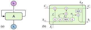
A RNN (recurrent neural network) is a kind of deep neural network for processing sequence data considering the impact of last moments on the present. Parameter sharing on a time domain with a loop structure is its important character. As shown in Fig. 2a, X_t represents the input characteristics at time t, A is the computing unit which is also known as the hidden layer, and h_t is the output value. The hidden layer controls the information conversion process of the sequence data. It fits the mapping relations between the input multidimensional features and the labels and learns the weight matrix and bias to calculate the corresponding output value. However, RNN suffers from vanishing gradient or gradient explosion problems when dealing with long-term time-series data.

Table 1 Details of the experimental settings.

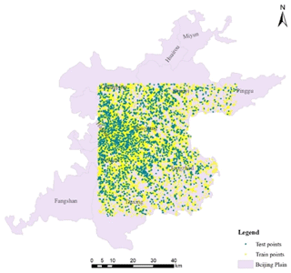
Figure 4 The distribution of the train and test data (the administrative map is from the Beijing Institute of Geo-Environment Monitoring).

The LSTM proposed by Hochreiter and Schmidhuber (1997) is a computing unit in a RNN structure. It introduced a gating function to avoid the long-term dependency problem. As shown in Fig. 2b, f_t, i_t, and o_t are three non-linear gate functions and named the forget gate, input gate, and output gate in each memory block, respectively. The key to the LSTM is the cell state C_t, which has only a small amount of linear interaction during the entire operation. It can effectively record history information for a long time through the three gates. For an input vector x_t, the calculation equations for an LSTM unit with the three gates are as follows:

$$\begin{array}{}\text{(1)}& {\displaystyle }{\mathit{f}}_t=\mathit{\sigma }({\mathbf{W}}_{\mathrm{f}}\cdot \left[{\mathit{h}}_{t\text{-}\mathrm{1}},{\mathit{x}}_t\right]+{\mathit{b}}_{\mathrm{f}}),\text{(2)}& {\displaystyle }{\mathit{i}}_t=\mathit{\sigma }({\mathbf{W}}_{\mathrm{i}}\cdot \left[{\mathit{h}}_{t\text{-}\mathrm{1}},{\mathit{x}}_t\right]+{\mathit{b}}_{\mathrm{i}}),\text{(3)}& {\displaystyle }{\mathit{o}}_t=\mathit{\sigma }({\mathbf{W}}_{\mathrm{o}}\cdot \left[{\mathit{h}}_{t\text{-}\mathrm{1}},{\mathit{x}}_t\right]+{\mathit{b}}_{\mathrm{o}}),\text{(4)}& {\displaystyle }{\mathit{C}}_t={\mathit{f}}_t\times {\mathit{C}}_{t\text{-}\mathrm{1}}+{\mathit{i}}_t\times {\stackrel{\mathrm{̃}}{\mathit{C}}}_t,\text{(5)}& {\displaystyle }{\stackrel{\mathrm{̃}}{\mathit{C}}}_t=\tanh ({\mathbf{W}}_{\mathrm{C}}\cdot \left[{\mathit{h}}_{t\text{-}\mathrm{1}},{\mathit{x}}_t\right]+{\mathit{b}}_{\mathrm{C}}),\text{(6)}& {\displaystyle }{\mathit{h}}_t={\mathit{o}}_t\times \tanh \left({\mathit{C}}_t\right),\end{array}$$

where W_f, W_i, W_o, and W_C are the weight matrices for input vectors and b_f, b_i, b_o, and b_C are the bias vectors at time t, respectively. ${\stackrel{\mathrm{̃}}{\mathit{C}}}_t$ is the cell state of x_t involving the hidden state value h_t-1 from a previous block at time t-1. C_t is the current unit state controlled by f_t and i_t. h_t is the current output value controlled by the output gate and the current unit state. σ and tanh are the activation functions, a non-linear calculation process.

Table 2 The RMSE of the 14 validation points.

Figure 5 The fit curve between modelled and InSAR-derived change in land subsidence.

3.3 Subsidence modelling

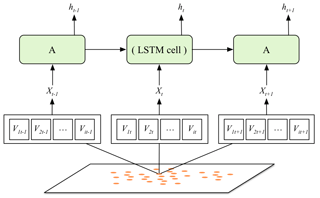
The LSTM model structure established in this study was drawn in Fig. 3. The orange dots are the PS points, which record the time-series land subsidence derived from synthetic aperture radar (SAR) images and corresponding attributes that influence the land subsidence. The green block which contains the LSTM computing cell is the memory block of the RNN model. X_t = {V_1t, V_2t, V_it} are the input data at time t. V_it is the ith attribute of each PS point at time t. The model would extract the characteristics of the multiple attributes through the time-series data from the input samples.

In this study, X_t = {V_1t, V_2t, V_3t, V_4t} = {the change in land subsidence, the change in confined groundwater level, compressible layer thickness, permeability coefficient}. It was a four-dimensional vector. The subsidence data were as the input labels and the attribute data were as the input features in the model-learning period. The model simulates the relationships between the change in subsidence and influencing factors.

Figure 6 The deviation between the modelled and InSAR-derived cumulative land subsidence at the last moment.

4 Results and discussion

4.1 Experimental settings

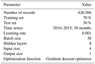
The detailed experimental settings are listed in Table 1. The datasets were randomly divided into 70 % for the training set and 30 % for the test set to verify the accuracy of the model. The distribution of these data is shown in Fig. 4. The model training stage used the sum of variance between the modelled and accurate values to calculate the loss. The gradient descent optimizer was used for the parameter optimization. The activation function was the common one Tanh. Limited by the data volume, the learning rate was set to 0.001 and the hidden layers were set to eight. A higher value can be set when the data volume is larger.

4.2 Experimental results

We got 13 190 points, in total 501 220 records as the training data, and 3297 points, in total 125 286 records, to test the model.

4.2.1 Results of LSTM modelling

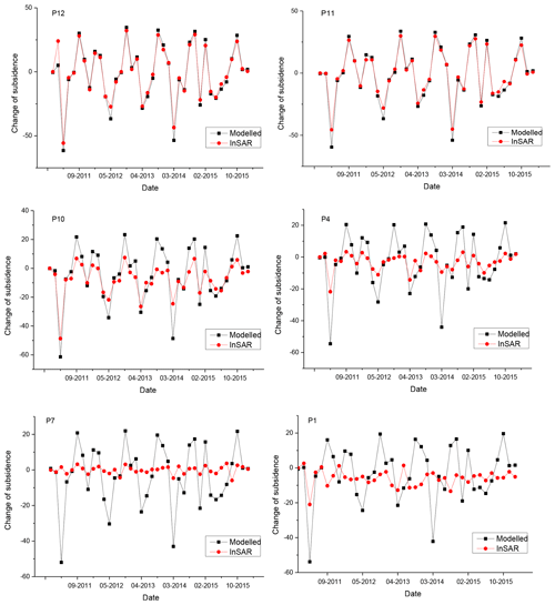
To evaluate the performance of the model, 12 PS points were selected randomly as the validation point (the black triangle legend in Fig. 1). We compared the modelled land subsidence with the InSAR-derived results and evaluated the errors with root-mean-square error (RMSE). As shown in Table 2, the southern points (P11, P12) with less of a cumulative subsidence have a small error, while those points located in the severe land subsidence areas (P1, P3, P5, P6, P7) have a high RMSE.

To evaluate the impact of land subsidence severity on the model results, we chose P11 and P12 located in the southern area where the subsidence is small, P4 and P10 at the edges of the subsidence regions and P1 and P7 in the severe land subsidence areas. The fitting curves between the modelled and InSAR-derived land subsidence of these points were plotted in Fig. 5.

The results show that the LSTM model performed well in areas where the subsidence is slight but poorly in places with severe subsidence.

Overall, the RMSE and MAE are 14.412 and 10.539, respectively. Notably, the results recorded the change in land subsidence, which means that the RMSE represented the error of the change in land subsidence.

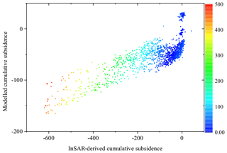
We calculated the change amount of land subsidence back to a cumulative quantity to assess the accuracy of the modelled cumulative land subsidence. The RMSE is 67.599. Figure 6 plotted the deviation between the modelled and InSAR-derived cumulative land subsidence. The deviation is small when the cumulative land subsidence is less than 100 mm. As the land subsidence increases, the deviation increases.

4.2.2 Analysis of the error source

As the results show, the severe land subsidence regions got a poor fit. These are areas of intense human activities (e.g. urban construction) and complex hydrogeological conditions, which are not reflected completely in the model.

There are two main error sources. One comes from inaccurate data and the selection of the input variables. In this study, we chose the confined groundwater level, the compressible layer thickness and the permeability coefficient as the influencing factors. The input groundwater level data were interpolated by the kriging method which may ignore the influence of the geological environment. The permeability coefficient has very little impact on the result. The selection of the input variables should include the main factors that affect land subsidence, such as the compressibility. These data are unpublished in our study area. It may be inverse to geotechnical test and geophysical methods in the future.

The other comes from the imperfect method. The LSTM model can process the time-series data well, but cannot deal with spatial phenomena. However, besides the groundwater level, the other two factors are almost constant in the time domain and spatially heterogeneous. This may be solved by combining the convolutional neural network (CNN) model which can extract spatial characteristics. In addition, the LSTM extracts characteristics from data, ignoring the physical process of land subsidence. This may also reduce its accuracy.

5 Conclusion and future work

This study constructed an LSTM model to simulate the land subsidence using the PS data detected by InSAR technology. Three factors were considered, which are the change in confined groundwater level, compressible layer thickness, and permeability coefficient. The model performed well in the southern areas where the subsidence is slight but poorly in the northern places with severe land subsidence. Land subsidence is a temporal–spatial phenomenon, and the LSTM model is a data analysis method with no consideration of physical mechanisms. In the future, we should combine the CNN model to solve the spatial heterogeneity and consider the physical process such as the consolidation theory in the model. Compared with the numerical simulation model and other grey models, this method requires fewer hydrogeological parameters and can be used for long-term large-area land subsidence modelling.