Effect of the water stress on gross primary production modeling of a Mediterranean oak savanna ecosystem

Dehesa ecosystem consists of widely-spaced oak trees combined with crops, pasture and Mediterranean shrubs. It is located in the southwest of the Iberian Peninsula, where water scarcity is recurrent, severely affecting the multiple productions and services of the ecosystem. Upscaling in situ Gross Primary Production (GPP) estimates in these areas is challenging for regional and global studies, given the significant spatial variability of plant functional types and the vegetation stresses usually present. The estimation of GPP is often addressed using light use efficiency models (LUE-models). Under soil water deficit conditions, biomass production is reduced below its potential rate. This work investigates the effect of different parameterizations to account for water stress on GPP estimates and their agreement with observations. Ground measurements of GPP are obtained using an Eddy Covariance (EC) system installed over an experimental site located in Córdoba, Spain. GPP is estimated with a LUE-model in the footprint of the EC tower using several approaches: a fixed value taken from previous literature; a fixed value modified by daily weather conditions; and both formulations modified by an additional coefficient to explicitly consider the vegetation water stress. The preliminary results obtained during two hydrological years (2015/2016 and 2016/2017) are compared, focusing on specific wet and dry periods.

1 Introduction

Dehesa (known as montado in Portugal) ecosystem combines forest, agricultural and extensive livestock productions, presenting important ecosystem services and cultural values. It is composed of sparse trees (mainly holm oak) and an undergrowth of shrub, pasture or herbaceous crop, constituting a characteristic landscape of the southwest of the Iberian Peninsula (Parsons, 1962).

This landscape is characterized by the low fertility of the soils, not suitable for regular farming, and a Mediterranean climate with a high vulnerability to global warming, with increasingly extreme droughts and torrential rainfalls (Kovats et al., 2014).

The assimilation of CO₂ due to the vegetation is represented by the gross primary production (GPP). This production is often estimated from remote sensing based on the works of Monteith (1972) that use biophysical variables and subsequently validated with eddy covariance (EC) systems (e.g. Migliavacca et al., 2009; Wagle et al., 2014; Zhang et al., 2015). These models, known as light use efficiency (LUE) models, relate the incident solar radiation with the photosynthetic activity of the plant, or canopy, through a LUE parameter, which is the amount of biomass produced per unit of radiation absorbed. Under soil water deficit conditions, biomass production is reduced below its potential rate, but this effect is sometimes addressed only indirectly by these models.

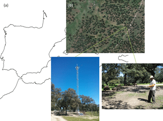
Figure 1 Study site (a), Aerial photography of the area (b), EC tower (c) and field measurements example (d).

The objective of this work is to test different approaches to consider water stress on GPP estimates over a dehesa ecosystem using a LUE-model. GPP has been estimated with a LUE-model using field data, Sentinel-2 images, meteorological information and several LUE approaches: a fixed value; a fixed value modified by daily weather conditions; and both formulations with an additional coefficient to explicitly consider the vegetation water stress. The results were compared to those obtained from an EC system from July 2015 to September 2017, analyzing the behavior of the selected approaches at different temporal scales.

2 Material and methods

2.1 Study site and eddy covariance data

The study site is a farm located in Cardeña (Córdoba, Spain) (Fig. 1a), part of an environmental protected area. It presents an average rainfall of 720 (±150) mm per year, cold winters, long and dry summers and periodic severe droughts.

The EC system is installed in a gently sloped area with uniform fetch (length in the prevailing wind direction) and homogeneous vegetation (holm oak and pasture) (Fig. 1b and c). The equipment is located at 18 m above ground level in order to minimize the effect of roughness (trees present 7-8 meters of height). A limited number of available measurements caused by a loss of data of the EC tower during one month occurred in the first trimester of 2016. GPP was estimated using Eq. (1):

$$\begin{array}{}\text{(1)}& {\displaystyle }{\displaystyle }\mathrm{GPP}=\mathrm{NEE}-R_{\mathrm{eco}}\end{array}$$

where NEE is the net ecosystem exchange given by the EC and R_eco is the respiration of the heterotrophic part of the ecosystem which was calculated by a day-time based flux-partitioning algorithm (Lasslop et al., 2010).

2.2 Application of a LUE-model

The GPP was estimated using an adaptation of Monteith (1972) model (Eq. 2):

$$\begin{array}{}\text{(2)}& {\displaystyle }{\displaystyle }\mathrm{GPP}=\mathrm{fPAR}\mathrm{PAR}\mathit{\epsilon }\end{array}$$

where GPP (g m⁻²) is the gross primary production, fPAR (dimensionless) is the fraction of photosynthetically active radiation absorbed by the vegetation, PAR (MJ m⁻²) is the photosynthetically active radiation and ε (g MJ⁻¹) is the light use efficiency.

2.2.1 Estimation of fPAR

Sentinel-2 images and field measurements have been combined to estimate fPAR. A set of 55 Sentinel-2 cloud-free images were selected (Fig. 2a) and the NDVI was calculated using bands 4 (red) and 8 (NIR) (Fig. 2b) for the study period. The resulting images were linearly interpolated pixel by pixel to obtain a daily NDVI image with 10 m of spatial resolution.

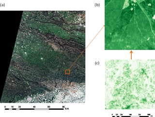
Figure 2 RGB Sentinel-2a image (7 April 2016) (a), NDVI (7 April 2016) (b) and fcover images (28 July 2017) (c).

For the transformation NDVI to fPAR, holm oaks and the pasture were addressed separately. For the holm oak, fPAR was monthly monitored by measuring 15 selected trees from the footprint area of the EC during the study period with a LP-80 ceptometer (Fig. 1d) and computing an average from these values that was used as constant value per month. For the pasture, it was used a linear relationship of NDVI-fPAR determined from satellite data in a previous study over the same area (Gómez-Giráldez et al., 2018). The separation between tree and pasture at pixel level was done assuming that the spectral response of both canopies is additive (e.g. Lu et al., 2003; Blanco et al., 2016). To differentiate the percentage of trees and pasture in each pixel, the coverage fraction image (fcover) was obtained using SNAP toolbox by ESA (http://step.esa.int/main/toolboxes/snap/, last access: 25 July 2018). The Sentinel-2 image of 28 July 2017 was used as reference (Fig. 2c). On this date, the pasture is totally dry and the fcover corresponded only to the tree canopy and can be considered constant.

With these premises, Eq. (3) was obtained:

$$\begin{array}{}\text{(3)}& {\displaystyle }{\displaystyle }\mathrm{fPAR}={\mathrm{fPAR}}_{\mathrm{oak}}\mathrm{fcover}+{\mathrm{fPAR}}_{\mathrm{pasture}}(\mathrm{1}-\mathrm{fcover}).\end{array}$$

Finally, to obtain a daily value representative of EC footprint area, a daily footprint function was calculated and used to weigh image pixels. The final data is the sum of the product of fPAR and footprint weights.

2.2.2 Estimation of PAR

The PAR estimation is computed using daily values of solar radiation measured with a 4-component net radiometer NR-1 and a reducing factor of 0.48 according to Szeicz (1974), obtained from measurements in a set of points distributed throughout the globe.

Figure 3 Temporal profile of the GPP fluxes: (a) EC, max and meteo (b) EC, W and all.

2.2.3 Estimation of ε

A maximum value (ε_max) of 0.77 was selected, based on the results obtained by Running et al. (2000) for wooded grassland. Four methods were analysed:

1. Max: the use of ε_max to test the need to attenuate it.

2. Meteo: it uses the attenuation proposed by Running et al. (2000) considering the climatic variables that reduce the efficiency of the plant: minimum daily temperature (T_min) and the vapour pressure deficit (VPD). A scalar minimum temperature and the scalar VPD, which are simple linear ramp functions between 0 and 1 derived from the daily values of T_min and VPD. These linear function are obtained using threshold values, where the minimum and maximum value for T_min correspond to 0 and 1 vales of scalar T_min (increasing function) respectively; and minimum and maximum value for VPD correspond to 1 and 0 vales of scalar VPD (decreasing function respectively). The threshold values used were: −8 and 11.39 ^∘C for T_min, and 0.65 and 3.1 kPa for VPD.

3. W: the use of an attenuation factor due to the water stress of the ecosystem computed by Eq. (4):

   $$\begin{array}{}\text{(4)}& {\displaystyle }{\displaystyle }W={\displaystyle \frac{\mathrm{ET}}{{\mathrm{ET}}_{\mathrm{r}}}}\end{array}$$

   where W (dimensionless) is the water stress coefficient multiplying ε_max value; ET (mm day⁻¹) is the daily evapotranspiration of the system by the method of Bowen (1926); and ET_r (mm day⁻¹) is the reference evapotranspiration estimated by the Hargreaves formula (Hargreaves and Samani, 1985).

4. All: this approach consider the application of the two previous attenuations, reducing the ε_max by multiplying both, W and the scalar VPD and T_min.

All the meteorological data required for the calculations were obtained from half-hour measurements of the EC system.

2.3 Study of the methods

In order to study the 4 methods at different temporal scales, the correlation coefficient (R²) of the linear regressions, the root mean squared error (RMSE) and the Mean Absolute Percentage error (MAPE) of the four methods were calculated at different temporal scales: (i) daily data was analysed for the entire study period; (ii) average values were computed for each of the two hydrological years (1 October to 30 September) 2015/2016 and 2016/2017; (iii) data was averaged in terms of wet (1 October to 15 May) and dry periods (15 May to 30 September).

Finally, the accumulated values for each hydrological year and period were obtained and compared to the measurements of the EC.

3 Results and discussion

The values obtained for fPAR and W for the area vary between 0.2 and 0.7, and 0.03 and 1.10, respectively with average values for the study period of 0.44 and 0.38. Both variables presented a high variability, representative of the Mediterranean climate and vegetation. The average values for ε along the study period were: 0.3 g MJ⁻¹ for meteo method, 0.29 g MJ⁻¹ for W method and 0.14 for all method.

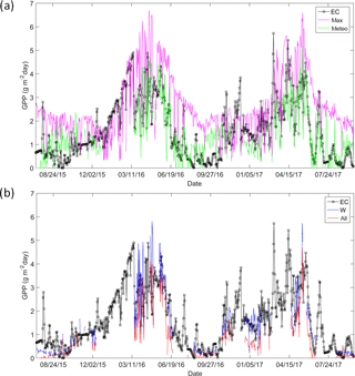
Figure 3 shows the temporal profile of GPP at daily scale obtained by the EC and estimated with the four methods considered. The seasonal variation of GPP along the study period can be appreciated, with clear differences between wet and dry periods.

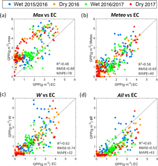
Figure 4 Comparison of GPP measured by the EC vs. max (a), EC vs. meteo (b), EC vs. W (c) and EC vs. all (d). Blue: wet period; orange: dry period; circle: 2015/2016; triangle: 2016/2017; black line: 1:1 line.

The method max (Fig. 4a) presented the weakest correlation (0.48) as expected, the highest error (RMSE = 0.88g m⁻²; MAPE = 78 %) and a general overestimation. The meteo method (Fig. 4b) improved the results which were similar to those of the W method (Fig. 4c) with no significant biases. Finally, despite the method all (Fig. 4d) underestimated the GPP (MAPE = 43 %), it presented the best correlation (0.65) and lower RMSE (0.51 g m⁻²). The correlation values obtained using W were lower than those obtained previously by Gilabert et al. (2015), but this difference could be explained by the significant higher spatial resolution of this analysis, 10 m, compared to the aggregation at 1 km of their study.

It can be appreciated that there are very low values in summer when the photosynthetic activity is lower. The pasture is dry and not contributing, and the stomata of the trees are often closed. The methods W and all performed poorly in this range of very low GPP values. The other cases (max and meteo) did not present this effect because they overestimated GPP.

The results obtained for both hydrological years (Table 1) were of similar order of magnitude.

The results obtained during the wet periods (Table 1) presented the poorest correlations. The 2016/2017 wet period presented an analogous behaviour, in terms of correlations and errors, compared to that obtained with the whole hydrological year but with lower correlation values. However, the 2015/2016 wet period showed a similar correlation value (around 0.4) in all methods possibly due to the gap in EC.

The results for the dry periods showed the highest correlation (over 0.8 and 0.7 in 2016 and 2017 respectively) but with higher dispersion (higher MAPE than wet period) and the use of the water stress factor improved the results. This difference between the periods confirms the findings of previous studies (e.g. Heinsch et al., 2006).

Finally, Table 2 presents the accumulated GPP values and the differences in percentage with respect to the EC data.

Table 1 R², RMSE (g m⁻²) and MAPE (%) obtained by comparison with EC measurements for 2015/2016 and 2016/2017 in the four methods, and over wet and dry periods.

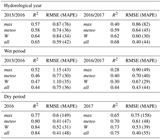
Table 2 Accumulated GPP (g m⁻² day⁻¹) for hydrological year and wet and dry period. The percentage represents the difference respect to EC data.

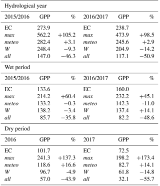
Comparing the accumulated GPP the max method strongly overestimated the GPP, in both dry periods (around 150 %) and wet periods (around 50 %). All underestimated about a 45 % independently dry or wet period. Meteo attenuation results obtained for hydrological year and especially for wet period were the most accurate (11 % or less). W attenuation was the most accurate for dry periods (differences lower than 15 %), results that agree with other studies as Dong et al. (2015).

4 Conclusions

This study explored different approaches to estimate GPP considering environmental factors and present a preliminary assessment of four different methods. On a daily scale, the combined use of a water stress index and meteorological attenuation provided better GPP estimates regarding R² and RMSE than the other formulations, especially for the dry season. However, this method presented a bias at daily scale that for the accumulated values resulted in a significant underestimation of seasonal values.

The use of a fixed value of ε presented the poorest results, supporting the need for environmental attenuation factors, as the approaches tested here. Meteo and W provided similar estimates, even when the nature of the attenuation considered was different. Further analysis of these factors is required to propose a specific model suited to dehesa ecosystem.